Tetration

Not to be confused with Titration, a procedure in chemistry.

In mathematics, tetration (also known as hyper-4) is an iterated exponential and is the next hyper operator after exponentiation. The word tetration was coined by English mathematician Reuben Louis Goodstein from tetra- (four) and iteration. Tetration is used for the notation of very large numbers. Shown here are examples of the first four hyper operators, with tetration as the fourth (and succession, the unary operation denoted $a' = a %2B 1$ taking $a$ and yielding the number after $a$ , as the 0th):

Addition

$a %2B n = a\!\underbrace{''{}^{\cdots}{}'}_n$

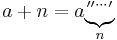
a succeeded n times.
Multiplication

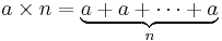
$a \times n = \underbrace{a %2B a %2B \cdots %2B a}_n$

a added to itself, n times.
Exponentiation

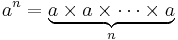
$a^n = \underbrace{a \times a \times \cdots \times a}_n$

a multiplied by itself, n times.
Tetration

${^{n}a} = \underbrace{a^{a^{\cdot^{\cdot^{a}}}}}_n$

a exponentiated by itself, n times.

where each operation is defined by iterating the previous one (the next operation in the sequence is pentation). The peculiarity of the tetration among these operations is that the first three (addition, multiplication and exponentiation) are generalized for complex values of n, while for tetration, no such regular generalization is yet established; and tetration is not considered an elementary function.

Addition (a + n) is the most basic operation, multiplication (an) is also a primary operation, though for natural numbers it can be thought of as a chained addition involving n numbers a, and exponentiation ( $a^n$ ) can be thought of as a chained multiplication involving n numbers a. Analogously, tetration ( $^{n}a$ ) can be thought of as a chained power involving n numbers a. The parameter a may be called the base-parameter in the following, while the parameter n in the following may be called the height-parameter (which is integral in the first approach but may be generalized to fractional, real and complex heights, see below).

Definition

For any positive real $a > 0$ and non-negative integer $n \ge 0$ , we define $\,\! {^{n}a}$ by:

${^{n}a}�:= \begin{cases} 1 &\text{if }n=0 \\ a^{\left[^{(n-1)}a\right]} &\text{if }n>0 \end{cases}$

Iterated powers

As we can see from the definition, when evaluating tetration expressed as an "exponentiation tower", the exponentiation is done at the deepest level first (in the notation, at the highest level). In other words:

$\,\!\ ^{4}2 = 2^{2^{2^2}} = 2^{\left[2^{\left(2^2\right)}\right]} = 2^{\left(2^4\right)} = 2^{16} = 65,\!536$

Note that exponentiation is not associative, so evaluating the expression in the other order will lead to a different answer:

$\,\! 2^{2^{2^2}} \ne \left[{\left(2^2\right)}^2\right]^2 = 2^{2 \cdot 2 \cdot2} = 256$

Thus, the exponential towers must be evaluated from top to bottom (or right to left). Computer programmers refer to this choice as right-associative.

When a and n are coprime, we can compute the last m decimal digits of $\scriptstyle\underbrace{a^{a^{\cdot^{\cdot^{a}}}}}_n$ using Euler's Theorem.

Terminology

There are many terms for tetration, each of which has some logic behind it, but some have not become commonly used for one reason or another. Here is a comparison of each term with its rationale and counter-rationale.

The term tetration, introduced by Goodstein in his 1947 paper Transfinite Ordinals in Recursive Number Theory^[1] (generalizing the recursive base-representation used in Goodstein's theorem to use higher operations), has gained dominance. It was also popularized in Rudy Rucker's Infinity and the Mind.
The term superexponentiation was published by Bromer in his paper Superexponentiation in 1987.^[2] It was used earlier by Ed Nelson in his book Predicative Arithmetic, Princeton University Press, 1986.
The term hyperpower^[3] is a natural combination of hyper and power, which aptly describes tetration. The problem lies in the meaning of hyper with respect to the hyper operator hierarchy. When considering hyper operators, the term hyper refers to all ranks, and the term super refers to rank 4, or tetration. So under these considerations hyperpower is misleading, since it is only referring to tetration.
The term power tower^[4] is occasionally used, in the form "the power tower of order n" for ${\ \atop {\ }} {{\underbrace{a^{a^{\cdot^{\cdot^{a}}}}}} \atop n}$

Tetration is often confused with closely related functions and expressions. This is because much of the terminology that is used with them can be used with tetration. Here are a few related terms:

Form	Terminology
$a^{a^{\cdot^{\cdot^{a^a}}}}$	Tetration
$a^{a^{\cdot^{\cdot^{a^x}}}}$	Iterated exponentials
$a_1^{a_2^{\cdot^{\cdot^{a_n}}}}$	Nested exponentials (also towers)
$a_1^{a_2^{a_3^{\cdot^{\cdot^\cdot}}}}$	Infinite exponentials (also towers)

In the first two expressions a is the base, and the number of times a appears is the height (add one for x). In the third expression, n is the height, but each of the bases is different.

Care must be taken when referring to iterated exponentials, as it is common to call expressions of this form iterated exponentiation, which is ambiguous, as this can either mean iterated powers or iterated exponentials.

Notation

There are many different notation styles that can be used to express tetration. Some of these styles can be used for higher iterations as well (hyper-5, hyper-6, and so on).

Name	Form	Description
Standard notation	$\,{}^{n}a$	Used by Maurer [1901] and Goodstein [1947]; Rudy Rucker's book Infinity and the Mind popularized the notation.
Knuth's up-arrow notation	$a {\uparrow\uparrow} n$	Allows extension by putting more arrows, or, even more powerfully, an indexed arrow.
Conway chained arrow notation	$a \rightarrow n \rightarrow 2$	Allows extension by increasing the number 2 (equivalent with the extensions above), but also, even more powerfully, by extending the chain
Ackermann function	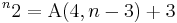${}^{n}2 = \operatorname{A}(4, n - 3) %2B 3$	Allows the special case $a=2$ to be written in terms of the Ackermann function.
Iterated exponential notation	${}^{n}a = \exp_a^n(1)$	Allows simple extension to iterated exponentials from initial values other than 1.
Hooshmand notation^[5]	$\operatorname{uxp}_a n, \, a^{\frac{n}{}}$
Hyper operator notation	$a^{(4)}n, \, \operatorname{hyper}_4(a,n)$	Allows extension by increasing the number 4; this gives the family of hyper operations
ASCII notation	`a^^n`	Since the up-arrow is used identically to the caret (`^`), the tetration operator may be written as (`^^`).

One notation above uses iterated exponential notation; in general this is defined as follows:

$\exp_a^n(x) = a^{a^{\cdot^{\cdot^{a^x}}}}$ with n "a"s.

There are not as many notations for iterated exponentials, but here are a few:

Name	Form	Description
Standard notation	$\exp_a^n(x)$	Euler coined the notation $\exp_a(x) = a^x$ , and iteration notation $f^n(x)$ has been around about as long.
Knuth's up-arrow notation	$(a{\uparrow})^n(x)$	Allows for super-powers and super-exponential function by increasing the number of arrows; used in the article on large numbers.
Ioannis Galidakis' notation	$\,{}^{n}(a, x)$	Allows for large expressions in the base.^[6]
ASCII (auxiliary)	`a^^n@x`	Based on the view that an iterated exponential is auxiliary tetration.
ASCII (standard)	`exp_a^n(x)`	Based on standard notation.
J Notation	`x^^:(n-1)x`	Repeats the exponentiation. See J (programming language)^[7]

Examples

In the following table, most values are too large to write in scientific notation, so iterated exponential notation is employed to express them in base 10. The values containing a decimal point are approximate.

$x$	${}^{2}x$	${}^{3}x$	${}^{4}x$
1	1	1	1
2	4	16	65,536
3	27	7,625,597,484,987	$\exp_{10}^3(1.09902)$
4	256	$\exp_{10}^2(2.18788)$	$\exp_{10}^3(2.18726)$
5	3,125	$\exp_{10}^2(3.33931)$	$\exp_{10}^3(3.33928)$
6	46,656	$\exp_{10}^2(4.55997)$	$\exp_{10}^3(4.55997)$
7	823,543	$\exp_{10}^2(5.84259)$	$\exp_{10}^3(5.84259)$
8	16,777,216	$\exp_{10}^2(7.18045)$	$\exp_{10}^3(7.18045)$
9	387,420,489	$\exp_{10}^2(8.56784)$	$\exp_{10}^3(8.56784)$
10	10,000,000,000	$\exp_{10}^3(1)$	$\exp_{10}^4(1)$

Approximations by more primitive functions

Polynomial approximations

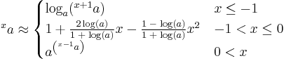
Linear approximation

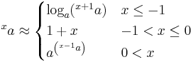
A linear approximation (solution to the continuity requirement, approximation to the differentiability requirement) is given by:

${}^{x}a \approx \begin{cases} \log_a(^{x%2B1}a) & x \le -1 \\ 1 %2B x & -1 < x \le 0 \\ a^{\left(^{x-1}a\right)} & 0 < x \end{cases}$

hence:

Approximation	Domain
$\,{}^{x}a \approx x%2B1$	for $-1<x<0$
$\,{}^{x}a \approx a^x$	for $0<x<1$
$\,{}^{x}a \approx a^{a^{(x-1)}}$	for $1<x<2$

and so on. However, it is only piecewise differentiable; at integer values of x the derivative is multiplied by $\ln{a}$ .

Examples

$\begin{align} {}^{\frac{1}{2}\pi}e &\approx 5.868...,\\ {}^{-4.3}0.5 &\approx 4.03335... \end{align}$

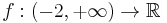A main theorem in Hooshmand's paper^[5] states: Let $0 <a \neq 1$ . If $f:(-2,%2B\infty)\rightarrow \mathbb{R}$ is continuous and satisfies the conditions:

$f(x)=a^{f(x-1)} \; \; \mbox{for all} \; \; x>-1, \; f(0)=1$ ,
$f$ is differentiable on $(-1, 0)$ ,
$f^\prime$ is a nondecreasing or nonincreasing function on $(-1,0),$
$f^\prime (0^%2B) = (\ln a) f^\prime (0^-) \mbox{ or } f^\prime (-1^%2B) = f^\prime (0^-).$

then $f$ is uniquely determined through the equation

$f(x)=\exp^{[x]}_a (a^{x})=\exp^{[x%2B1]}_a(x) \quad \mbox{for all} \; \; x > -2$ ,

where $(x)=x-[x]$ denotes the fractional part of x and $\exp^{[x]}_a$ is the $[x]$ -iterated function of the function $\exp_a$ .

The proof is that the second through fourth conditions trivially imply that f is a linear function on [-1, 0].

The linear approximation to natural tetration function ${}^xe$ is continuously differentiable, but its second derivative does not exist at integer values of its argument. Hooshmand derived another uniqueness theorem for it which states:

If $f: (-2, %2B\infty)\rightarrow \mathbb{R}$ is a continuous function that satisfies:

$f(x)=e^{f(x-1)} \; \; \mbox{for all} \; \; x>-1, \; f(0)=1$ ,
$f$ is convex on $(-1,0)$ ,
$f^\prime (0^-)\leq f^\prime (0^%2B).$

then $f=\mbox{uxp}$ . [Here $f=\mbox{uxp}$ is Hooshmand's name for the linear approximation to the natural tetration function.]

The proof is much the same as before; the recursion equation ensures that $f^\prime (-1^%2B) = f^\prime (0^%2B),$ and then the convexity condition implies that $f$ is linear on (-1, 0).

Therefore the linear approximation to natural tetration is the only solution of the equation 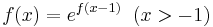$f(x)=e^{f(x-1)} \; \; (x>-1)$ and $f(0)=1$ which is convex on $(-1,%2B\infty)$ . All other sufficiently-differentiable solutions must have an inflection point on the interval (-1, 0).

Higher order approximations

A quadratic approximation (to the differentiability requirement) is given by:

${}^{x}a \approx \begin{cases} \log_a({}^{x%2B1}a) & x \le -1 \\ 1 %2B \frac{2\log(a)}{1 \;%2B\; \log(a)}x - \frac{1 \;-\; \log(a)}{1 \;%2B\; \log(a)}x^2 & -1 < x \le 0 \\ a^{\left({}^{x-1}a\right)} & 0 < x \end{cases}$

which is differentiable for all $x > 0$ , but not twice differentiable. If $a = e$ this is the same as the linear approximation.

A cubic approximation and a method for generalizing to approximations of degree n are given at.^[8]

Extensions

Tetration can be extended to define ${^n 0}$ and other domains as well.

Extension of domain for bases

Extension to base zero

The exponential $0^0$ is non consistently defined. Thus, the tetrations $\,{^{n}0}$ are not clearly defined by the formula given earlier. However, $\lim_{x\rightarrow0} {}^{n}x$ is well defined, and exists:

$\lim_{x\rightarrow0} {}^{n}x = \begin{cases} 1, & n \mbox{ even} \\ 0, & n \mbox{ odd} \end{cases}$

Thus we could consistently define 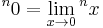${}^{n}0 = \lim_{x\rightarrow0} {}^{n}x$ . This is equivalent to defining $0^0 = 1$ .

Under this extension, ${}^{0}0 = 1$ , so the rule ${^{0}a} = 1$ from the original definition still holds.

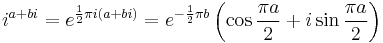
Extension to complex bases

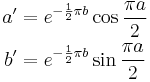
Since complex numbers can be raised to powers, tetration can be applied to bases of the form $\scriptstyle z \;=\; a %2B bi$ , where $\scriptstyle i$ is the square root of −1. For example, $\scriptstyle {}^{n}z$ where $\scriptstyle z \;=\; i$ , tetration is achieved by using the principal branch of the natural logarithm, and using Euler's formula we get the relation:

$i^{a%2Bbi} = e^{\frac{1}{2}{\pi i} (a%2Bbi)} = e^{-\frac{1}{2}{\pi b}} \left(\cos{\frac{\pi a}{2}} %2B i \sin{\frac{\pi a}{2}}\right)$

This suggests a recursive definition for 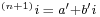$\scriptstyle {}^{(n%2B1)}i \;=\; a'%2Bb'i$ given any $\scriptstyle {}^{n}i \;=\; a%2Bbi$ :

$\begin{align} a' &= e^{-\frac{1}{2}{\pi b}} \cos{\frac{\pi a}{2}} \\ b' &= e^{-\frac{1}{2}{\pi b}} \sin{\frac{\pi a}{2}} \end{align}$

The following approximate values can be derived:

${}^{n}i$	Approximate Value
${}^{1}i = i$	i
${}^{2}i = i^{\left({}^{1}i\right)}$	$0.2079$
${}^{3}i = i^{\left({}^{2}i\right)}$	$0.9472 %2B 0.3208i$
${}^{4}i = i^{\left({}^{3}i\right)}$	$0.0501 %2B 0.6021i$
${}^{5}i = i^{\left({}^{4}i\right)}$	$0.3872 %2B 0.0305i$
${}^{6}i = i^{\left({}^{5}i\right)}$	$0.7823 %2B 0.5446i$
${}^{7}i = i^{\left({}^{6}i\right)}$	$0.1426 %2B 0.4005i$
${}^{8}i = i^{\left({}^{7}i\right)}$	$0.5198 %2B 0.1184i$
${}^{9}i = i^{\left({}^{8}i\right)}$	$0.5686 %2B 0.6051i$

Solving the inverse relation as in the previous section, yields the expected $\scriptstyle \,{}^{0}i \;=\; 1$ and $\scriptstyle \,{}^{(-1)}i \;=\; 0$ , with negative values of n giving infinite results on the imaginary axis. Plotted in the complex plane, the entire sequence spirals to the limit $0.4383 %2B 0.3606i$ , which could be interpreted as the value where n is infinite.

Such tetration sequences have been studied since the time of Euler but are poorly understood due to their chaotic behavior. Most published research historically has focused on the convergence of the power tower function. Current research has greatly benefited by the advent of powerful computers with fractal and symbolic mathematics software. Much of what is known about tetration comes from general knowledge of complex dynamics and specific research of the exponential map.

Extensions of the domain for (iteration) "heights"

Extension to infinite heights

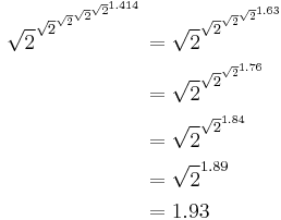
Tetration can be extended to infinite heights (n in ${}^{n}a$ ). This is because for bases within a certain interval, tetration converges to a finite value as the height tends to infinity. For example, $\sqrt{2}^{\sqrt{2}^{\sqrt{2}^{\cdot^{\cdot^{\cdot}}}}}$ converges to 2, and can therefore be said to be equal to 2. The trend towards 2 can be seen by evaluating a small finite tower:

$\begin{align} \sqrt{2}^{\sqrt{2}^{\sqrt{2}^{\sqrt{2}^{\sqrt{2}^{1.414}}}}} &= \sqrt{2}^{\sqrt{2}^{\sqrt{2}^{\sqrt{2}^{1.63}}}} \\ &= \sqrt{2}^{\sqrt{2}^{\sqrt{2}^{1.76}}} \\ &= \sqrt{2}^{\sqrt{2}^{1.84}} \\ &= \sqrt{2}^{1.89} \\ &= 1.93 \end{align}$

In general, the infinite power tower $x^{x^{\cdot^{\cdot^{\cdot}}}}$ , defined as the limit of ${}^{n}x$ as n goes to infinity, converges for e^−e ≤ x ≤ e^1/e, roughly the interval from 0.066 to 1.44, a result shown by Leonhard Euler. The limit, should it exist, is a positive real solution of the equation y = x^y. Thus, x = y^1/y. The limit defining the infinite tetration of x fails to converge for x > e^1/e because the maximum of y^1/y is e^1/e.

This may be extended to complex numbers z with the definition:

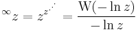
${}^{\infty}z = z^{z^{\cdot^{\cdot^{\cdot}}}} = \frac{\mathrm{W}(-\ln{z})}{-\ln{z}}$

where W(z) represents Lambert's W function.

As the limit y = ^∞x (if existent, i.e. for e^−e < x < e^1/e) must satisfy x^y = y we see that x ↦ y = ^∞x is (the lower branch of) the inverse function of y ↦ x = y^1/y.

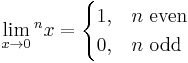
(Limited) extension to negative heights

In order to preserve the original rule:

${^{(k%2B1)}a} = a^{({^{k}a})}$

for negative values of $k$ we must use the recursive relation:

${^{k}a} = \log_a \left( {^{(k%2B1)}a} \right)$

Thus:

${}^{(-1)}a = \log_{a} \left( {}^{0}a \right) = \log_{a} 1 = 0$

However smaller negative values cannot be well defined in this way because

${}^{(-2)}a = \log_{a} \left( {}^{-1}a \right) = \log_{a} 0$

which is not well defined.

Note further that for $n = 1$ any definition of $\,\! {^{(-1)}1}$ is consistent with the rule because

${^{0}1} = 1 = 1^n$ for any $\,\! n = {^{(-1)}1}$ .

Extension to real heights

At this time there is no commonly accepted solution to the general problem of extending tetration to the real or complex values of $n$ . Various approaches are mentioned below.

In general the problem is finding, for any real a > 0, a super-exponential function $\,f(x) = {}^{x}a$ over real $x > -2$ that satisfies

$\,{}^{(-1)}a = 0$
$\,{}^{0}a = 1$
$\,{}^{x}a = a^{\left({}^{(x-1)}a\right)}$ for all real x > -1.
A fourth requirement that is usually one of:

A continuity requirement (usually just that ${}^{x}a$ is continuous in both variables for $x > 0$ ).
A differentiability requirement (can be once, twice, k times, or infinitely differentiable in x).
A regularity requirement (implying twice differentiable in x) that:

$\left( \frac{d^2}{dx^2}f(x) > 0\right)$ for all $x > 0$

The fourth requirement differs from author to author, and between approaches. There are two main approaches to extending tetration to real heights, one is based on the regularity requirement, and one is based on the differentiability requirement. These two approaches seem to be so different that they may not be reconciled, as they produce results inconsistent with each other.

Fortunately, any solution that satisfies one of these in an interval of length one can be extended to a solution for all positive real numbers. When $\,{}^{x}a$ is defined for an interval of length one, the whole function easily follows for all $x > -2$ .

Extension to complex heights

There is a conjecture^[9] that there exists a unique function F which is a solution of the equation F(z+1)=exp(F(z)) and satisfies the additional conditions that F(0)=1 and F(z) approaches the fixed points of the logarithm (roughly 0.31813150520476413531 ± 1.33723570143068940890i) as z approaches ±i∞ and that F is holomorphic in the whole complex z-plane, except the part of the real axis at z≤−2. This function is shown in the figure at right. The complex double precision approximation of this function is available online.^[10]

The requirement of holomorphism of tetration is important for the uniqueness. Many functions $S$ can be constructed as

$S(z)=F\!\left(~z~ %2B\sum_{n=1}^{\infty} \sin(2\pi n z)~ \alpha_n %2B\sum_{n=1}^{\infty} \Big(1-\cos(2\pi n z) \Big) ~\beta_n \right)$

where $\alpha$ and $\beta$ are real sequences which decay fast enough to provide the convergence of the series, at least at moderate values of $\Im(z)$ .

The function S satisfies the tetration equations S(z+1)=exp(S(z)), S(0)=1, and if α_n and β_n approach 0 fast enough it will be analytic on a neighborhood of the positive real axis. However, if some elements of {α} or {β} are not zero, then function S has multitudes of additional singularities and cutlines in the complex plane, due to the exponential growth of sin and cos along the imaginary axis; the smaller the coefficients {α} and {β} are, the further away these singularities are from the real axis.

The extension of tetration into the complex plane is thus essential for the uniqueness; the real-analytic tetration is not unique.

Inverse relations

Exponentiation has two inverse relations; roots and logarithms. Analogously, the inverse relations of tetration are often called the super-root, and the super-logarithm.

Super-root

For the album, see Super Roots.

The super-root is the inverse relation of tetration with respect to the base: if $^n y = x$ , then y is an nth super root of x. For example,

$^4 2 = 2^{2^{2^{2}}} = 65,536$

so 2 is the 4th super-root of 65,536 and

$^3 3 = 3^{3^{3}} = 7,625,597,484,987$

so 3 is the 3rd super-root (or super cube root) of 7,625,597,484,987.

Square super-root

The 2nd-order super-root, square super-root, or super square root has two equivalent notations, $\mathrm{ssrt}(x)$ and $\sqrt{x}_s$ . It is the inverse of $^2 x = x^x$ and can be represented with the Lambert W function:^[11]

$\mathrm{ssrt}(x)=e^{W(\mathrm{ln}(x))}=\frac{\mathrm{ln}(x)}{W(\mathrm{ln}(x))}$

Like square roots, the square super-root of x may not have a single solution. Unlike square roots, determining the number of square super-roots of x may be difficult. In general, if $e^{-1/e}<x<1$ , then x has two positive square super-roots between 0 and 1; and if $x > 1$ , then x has one positive square super-root greater than 1. If x is positive and less than $e^{-1/e}$ it doesn't have any real square super-roots, but the formula given above yields countably infinitely many complex ones for any finite x not equal to 1.^[11]

The super-root of two the solution to x^x=2 with the approximate value of 1.55961046946236935 is also the unique number whereas when put as the root of two and then as the logarithm of two the result is the same.

It is thought that if the square super-root of an integer is not an integer, it is irrational, but it is unknown if there is any proof for this.

Other super-roots

For each integer n > 2, the function ⁿx is defined and increasing for x ≥ 1, and ⁿ1 = 1, so that the nth super-root of x, $\sqrt[n]{x}_s$ , exists for x ≥ 1.

However, if the linear approximation above is used, then $^y x = y %2B 1$ if -1 < y ≤ 0, so $^y \sqrt{y %2B 1}_s$ cannot exist.

Other super-roots are expressible under the same basis used with normal roots: super cube roots, the function that produces y when $x = y^{y^y}$ , can be expressed as $\sqrt[3]{x}_s$ ; the 4th super-root can be expressed as $\sqrt[4]{x}_s$ ; and it can therefore be said that the n^th super-root is $\sqrt[n]{x}_s$ . Note that $\sqrt[n]{x}_s$ may not be uniquely defined, because there may be more than one n^th root. For example, x has a single (real) super-root if n is odd, and up to two if n is even.

The super-root can be extended to $n = \infty$ , and this shows a link to the mathematical constant e as it is only well-defined if 1/e ≤ x ≤ e (see extension of tetration to infinite heights). Note that $x = {^\infty y}$ implies that $x = y^x$ and thus that $y = x^{1/x}$ . Therefore, when it is well defined, $\sqrt[\infty]{x}_s = x^{1/x}$ and thus it is an elementary function. For example, $\sqrt[\infty]{2}_s = 2^{1/2} = \sqrt{2}$ .

Super-logarithm

Main article: Super-logarithm

Once a continuous increasing (in x) definition of tetration, ^xa, is selected, the corresponding super-logarithm slog_a x is defined for all real numbers x, and a > 1.

The function $\mathrm{slog}_a$ satisfies:

$\mathrm{slog}_a {^x a} = x$

$\mathrm{slog}_a a^x = 1 %2B \mathrm{slog}_a x$

$\mathrm{slog}_a x = 1 %2B \mathrm{slog}_a \log_a x$

$\mathrm{slog}_a x > -2$

The infra logarithm function is dual of the ultra exponential function and is denoted by $\mathrm{iog}_a$ . If $a>1$ , then it is inverse function of $\mathrm{uxp}_a$ .

References

^ R. L. Goodstein (1947). "Transfinite ordinals in recursive number theory". Journal of Symbolic Logic 12 (4): 123–129. doi:10.2307/2266486. JSTOR 2266486.
^ N. Bromer (1987). "Superexponentiation". Mathematics Magazine 60 (3): 169–174. JSTOR 2689566.
^ J. F. MacDonnell (1989). "Somecritical points of the hyperpower function $x^{x^{\dots}}$ ". International Journal of Mathematical Education 20 (2): 297–305. MR 994348. http://www.faculty.fairfield.edu/jmac/ther/tower.htm.
^ Weisstein, Eric W., "Power Tower" from MathWorld.
^ ^a ^b M. H. Hooshmand, (2006). "Ultra power and ultra exponential functions". Integral Transforms and Special Functions 17 (8): 549–558. doi:10.1080/10652460500422247.
^ Ioannis Galidakis. On Extending hyper4 and Knuth’s Up-arrow Notation to the Reals.
^ "Power Verb". J Vocabulary. J Software. http://www.jsoftware.com/help/dictionary/d202n.htm. Retrieved 28 October 2011.
^ Andrew Robbins. Solving for the Analytic Piecewise Extension of Tetration and the Super-logarithm.
^ D. Kouznetsov (July 2009). "Solution of $F(z%2B1)=\exp(F(z))$ in complex $z$ -plane". Mathematics of Computation 78 (267): 1647–1670. doi:10.1090/S0025-5718-09-02188-7. http://www.ams.org/mcom/2009-78-267/S0025-5718-09-02188-7/S0025-5718-09-02188-7.pdf.
^ Mathematica code for evaluation and plotting of the tetration and its derivatives.
^ ^a ^b Corless, R. M.; Gonnet, G. H.; Hare, D. E. G.; Jeffrey, D. J.; Knuth, D. E. (1996). "On the Lambert W function" (PostScript). Advances in Computational Mathematics 5: 333. doi:10.1007/BF02124750. http://www.apmaths.uwo.ca/~rcorless/frames/PAPERS/LambertW/LambertW.ps.

Daniel Geisler, tetration.org
Ioannis Galidakis, On extending hyper4 to nonintegers (undated, 2006 or earlier) (A simpler, easier to read review of the next reference)
Ioannis Galidakis, On Extending hyper4 and Knuth's Up-arrow Notation to the Reals (undated, 2006 or earlier).
Robert Munafo, Extension of the hyper4 function to reals (An informal discussion about extending tetration to the real numbers.)
Lode Vandevenne, Tetration of the Square Root of Two, (2004). (Attempt to extend tetration to real numbers.)
Ioannis Galidakis, Mathematics, (Definitive list of references to tetration research. Lots of information on the Lambert W function, Riemann surfaces, and analytic continuation.)
Galidakis, Ioannis and Weisstein, Eric W. Power Tower
Joseph MacDonell, Some Critical Points of the Hyperpower Function.
Dave L. Renfro, Web pages for infinitely iterated exponentials (Compilation of entries from questions about tetration on sci.math.)
R. Knobel. "Exponentials Reiterated." American Mathematical Monthly 88, (1981), p. 235-252.
Hans Maurer. "Über die Funktion $y=x^{[x^{[x(\cdots)]}]}$ für ganzzahliges Argument (Abundanzen)." Mittheilungen der Mathematische Gesellschaft in Hamburg 4, (1901), p. 33-50. (Reference to usage of $\ {^{n} a}$ from Knobel's paper.)
Marco Ripà, "La strana coda della serie n^n^...^n", Trento (2011). ISBN 9788861787896

Tetration

Contents

Definition

Iterated powers

Terminology

Notation

Examples

Approximations by more primitive functions

Polynomial approximations

Linear approximation

Examples

Higher order approximations

Extensions

Extension of domain for bases

Extension to base zero

Extension to complex bases

Extensions of the domain for (iteration) "heights"

Extension to infinite heights

(Limited) extension to negative heights

Extension to real heights

Extension to complex heights

Inverse relations

Super-root

Square super-root

Other super-roots

Super-logarithm

See also

References

External links