Square wave
A square wave is a kind of non-sinusoidal waveform, most typically encountered in electronics and signal processing. An ideal square wave alternates regularly and instantaneously between two levels. Its stochastic counterpart is a two-state trajectory.
Contents |
Origins and uses
Square waves are universally encountered in digital switching circuits and are naturally generated by binary (two-level) logic devices. They are used as timing references or "clock signals", because their fast transitions are suitable for triggering synchronous logic circuits at precisely determined intervals. However, as the frequency-domain graph shows, square waves contain a wide range of harmonics; these can generate electromagnetic radiation or pulses of current that interfere with other nearby circuits, causing noise or errors. To avoid this problem in very sensitive circuits such as precision analog-to-digital converters, sine waves are used instead of square waves as timing references.
In musical terms, they are often described as sounding hollow, and are therefore used as the basis for wind instrument sounds created using subtractive synthesis. Additionally, the distortion effect used on electric guitars clip the outermost regions of the waveform, causing it to increasingly resemble a square wave as more distortion is applied.
Simple two-level Rademacher functions are square waves.
Examining the square wave
In contrast to the sawtooth wave, which contains all integer harmonics, the square wave contains only odd integer harmonics.
Using Fourier series we can write an ideal square wave as an infinite series of the form
![\begin{align}
x_{\mathrm{square}}(t) & {} = \frac{4}{\pi} \sum_{k=1}^\infty {\sin{\left ([2k-1]2\pi ft \right )}\over(2k-1)} \\
& {} = \frac{4}{\pi}\left (\sin(2\pi ft) %2B {1\over3}\sin(6\pi ft) %2B {1\over5}\sin(10\pi ft) %2B \cdots\right )
\end{align}](/2012-wikipedia_en_all_nopic_01_2012/I/8297e8aa76fad645521cb416ae365afe.png)
A curiosity of the convergence of the Fourier series representation of the square wave is the Gibbs phenomenon. Ringing artifacts in non-ideal square waves can be shown to be related to this phenomenon. The Gibbs phenomenon can be prevented by the use of σ-approximation, which uses the Lanczos sigma factors to help the sequence converge more smoothly.
An ideal square wave requires that the signal changes from the high to the low state cleanly and instantaneously. This is impossible to achieve in real-world systems, as it would require infinite bandwidth. It would also require particles to be able to be able to travel faster than the speed of light, as the slope of an ideal square wave at these points is undefined (or infinite).
Even in the best approximation of a square wave, this slope is finite, however.
Real-world square-waves have only finite bandwidth, and often exhibit ringing effects similar to those of the Gibbs phenomenon, or ripple effects similar to those of the σ-approximation.
For a reasonable approximation to the square-wave shape, at least the fundamental and third harmonic need to be present, with the fifth harmonic being desirable. These bandwidth requirements are important in digital electronics, where finite-bandwidth analog approximations to square-wave-like waveforms are used. (The ringing transients are an important electronic consideration here, as they may go beyond the electrical rating limits of a circuit or cause a badly positioned threshold to be crossed multiple times.)
The ratio of the high period to the total period of a square wave is called the duty cycle. A true square wave has a 50% duty cycle - equal high and low periods. The average level of a square wave is also given by the duty cycle, so by varying the on and off periods and then averaging, it is possible to represent any value between the two limiting levels. This is the basis of pulse width modulation.
Characteristics of imperfect square waves
As already mentioned, an ideal square wave has instantaneous transitions between the high and low levels. In practice, this is never achieved because of physical limitations of the system that generates the waveform. The times taken for the signal to rise from the low level to the high level and back again are called the rise time and the fall time respectively.
If the system is overdamped, then the waveform may never actually reach the theoretical high and low levels, and if the system is underdamped, it will oscillate about the high and low levels before settling down. In these cases, the rise and fall times are measured between specified intermediate levels, such as 5% and 95%, or 10% and 90%. Formulas exist that can determine the approximate bandwidth of a system given the rise and fall times of the waveform.
Other definitions
The square wave has many definitions, which are equivalent except at the discontinuities:
It can be defined as simply the sign function of a sinusoid:
![\ x(t) = \sgn(\sin[t])](/2012-wikipedia_en_all_nopic_01_2012/I/5fb5245ad5aef8b523a79785b1d3bad8.png)
which will be 1 when the sinusoid is positive, −1 when the sinusoid is negative, and 0 at the discontinuities. It can also be defined with respect to the Heaviside step function u(t) or the rectangular function ⊓(t):
![\ x(t) = \sum_{n=-\infty}^{%2B\infty} \sqcap(t - nT) = \sum_{n=-\infty}^{%2B\infty} \left( u \left[t - nT %2B {1 \over 2} \right] - u \left[t - nT - {1 \over 2} \right] \right)](/2012-wikipedia_en_all_nopic_01_2012/I/0faaa4f7839a77543d24e02b7ebfee7d.png)
T is 2 for a 50% duty cycle. It can also be defined in a piecewise way:
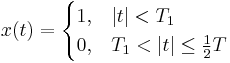
when