Split-quaternion

Coquaternion multiplication
×	1	i	j	k
1	1	i	j	k
i	i	−1	k	−j
j	j	−k	+1	−i
k	k	j	i	+1

In abstract algebra, the split-quaternions or coquaternions are elements of a 4-dimensional associative algebra introduced by James Cockle in 1849 under the latter name. Like the quaternions introduced by Hamilton in 1843, they form a four dimensional real vector space equipped with a multiplicative operation. Unlike the quaternion algebra, the split-quaternions contain zero divisors, nilpotent elements, and nontrivial idempotents. As a mathematical structure, they form an algebra over the real numbers, which is isomorphic to the algebra of 2 × 2 real matrices. The coquaternions came to be called split-quaternions due to the division into positive and negative terms in the modulus function. For other names for split-quaternions see the Synonyms section below.

The set $\{ 1, i, j, k \}$ forms a basis. The products of these elements are

$i j = k = -j i, \quad j k = -i = -k j, \quad k i = j = -i k,$

$i^2 = -1, \quad j^2 = %2B1, \quad k^2 = %2B1,$

and hence ijk = 1. It follows from the defining relations that the set 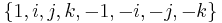$\{1, i, j, k, -1, -i, -j, -k\}$ is a group under coquaternion multiplication; it is isomorphic to the dihedral group of a square.

A coquaternion

$q~= w %2B x i %2B y j %2B z k$

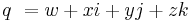
has a conjugate

$q^* ~= w - x i - y j - z k$

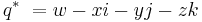
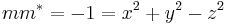
and multiplicative modulus

$qq^* ~= w^2 %2B x^2 - y^2 - z^2$ .

This quadratic form is split into positive and negative parts, in contrast to the positive definite form on the algebra of quaternions.

When the modulus is non-zero, then q has a multiplicative inverse, namely q*/qq*.

$U = \{q�: qq^* \ne 0 \}$

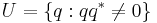
is the set of units. The set P of all coquaternions forms a ring (P, +, •) with group of units (U, •). The coquaternions with modulus qq* = 1 form a non-compact topological group SU(1,1), shown below to be isomorphic to SL(2,R).

The split-quaternion basis can be identified as the basis elements of either the Clifford algebra Cℓ_1,1(R), with {1, e₁=i, e₂=j, e₁e₂=k}; or the algebra Cℓ_2,0(R), with {1, e₁=j, e₂=k, e₁e₂=i}.

Historically coquaternions preceded Cayley's matrix algebra; coquaternions (along with quaternions and tessarines) evoked the broader linear algebra.

1 Matrix representations
2 Profile
3 Pan-orthogonality
4 Counter-sphere geometry
5 Application to kinematics
6 Historical notes
7 Synonyms
8 See also
9 References

Matrix representations

Let

$q = w %2B x i %2B y j %2B z k, ~ ~ u = w %2B x i, ~ ~ v = y %2B z i$

where u and v are ordinary complex numbers. Then the complex matrix

$\begin{pmatrix}u & v \\ v^* & u^* \end{pmatrix}$ ,

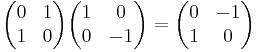
with $u^* = w - x i\ ,\ v^* = y - z i$ (complex conjugates of u and v), represents q in the ring of matrices in the sense that multiplication of split-quaternions behaves the same way as the matrix multiplication. For example, the determinant of this matrix is

$u u^* - v v^* = q q^*. \!$

The appearance of the minus sign, where there is a plus in H, distinguishes coquaternions from quaternions. The use of the split-quaternions of modulus one (q q* = 1) for hyperbolic motions of the Poincaré disk model of hyperbolic geometry is one of the great utilities of the algebra.

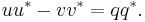
Besides the complex matrix representation, another linear representation associates coquaternions with 2 × 2 real matrices. This isomorphism can be made explicit as follows: Note first the product

$\begin{pmatrix} 0 & 1 \\ 1 & 0\end{pmatrix}\begin{pmatrix} 1 & 0 \\ 0 & -1\end{pmatrix} = \begin{pmatrix} 0 & -1 \\ 1 & 0\end{pmatrix}$

and that the square of each factor on the left is the identity matrix, while the square of the right hand side is the negative of the identity matrix. Furthermore, note that these three matrices, together with the identity matrix, form a basis for M(2,R). One can make the matrix product above correspond to j k = −i in the coquaternion ring. Then for an arbitrary matrix there is the bijection

$\begin{pmatrix} a & c \\ b & d\end{pmatrix} \leftrightarrow q = [(a%2Bd) %2B (c-b)i %2B (b%2Bc)j %2B (a-d)k]/2,$

which is in fact a ring isomorphism. Furthermore, computing squares of components and gathering terms shows that $q q^* = ad - bc \!$ , which is the determinant of the matrix. Consequently there is a group isomorphism between the unit quasi-sphere of coquaternions and SL2(R) = {g ∈ M(2,R) : det g = 1 }, and hence also with SU(1,1): the latter can be seen in the complex representation above.

For instance, see Karzel and Kist (1985) for the hyperbolic motion group representation with 2 × 2 real matrices.

Profile

The coquaternions may be given polar decomposition by delineation of subalgebras: Let

r(θ) = j cos θ + k sin θ (here θ is as fundamental as azimuth)

p(a, r) = i sinh a + r cosh a

v(a, r) = i cosh a + r sinh a

These are the equilateral-hyperboloidal coordinates described by Alexander Macfarlane.

Next, form three foundational sets in the vector-subspace of the ring:

E = { r ∈ P: r = r(θ), 0 ≤ θ < 2 π}

J = {p(a, r) ∈ P: a ∈ R, r ∈ E} catenoid

I = {v(a, r) ∈ P: a ∈ R, r ∈ E} hyperboloid of two sheets.

Now it is easy to verify that

{q ∈ P: q² = + 1} = J ∪ {1, -1}

and that

{q ∈ P: q² = −1} = I.

These set equalities mean that when p ∈ J then the plane

{x + yp: x, y ∈ R} = D_p

is a subring of P that is isomorphic to the plane of split-complex numbers just as when v is in I then

{x + yv: x, y ∈ R} = C_v

is a planar subring of P that is isomorphic to the ordinary complex plane C.

Note that for every r ∈ E, (r + i)² = 0 = (r − i)² so that r + i and r − i are nilpotents. The plane N = {x + y(r + i): x, y ∈ R} is a subring of P that is isomorphic to the dual numbers. Since every coquaternion must lie in a D_p, a C_v, or an N plane, these planes profile P. For example, the unit quasi-sphere

SU(1, 1) = {q ∈ P: qq* = 1}

consists of the "unit circles" in the constituent planes of P: In D_p it is a unit hyperbola, in N the "unit circle" is a pair of parallel lines, while in C_v it is indeed a circle (though it appears elliptical due to v-stretching).These ellipse/circles found in each C_v are like the illusion of the Rubin vase which "presents the viewer with a mental choice of two interpretations, each of which is valid".

Pan-orthogonality

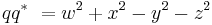
When coquaternion $q = w %2B xi %2B yj %2B zk$ , then the scalar part of q is w.
Definition: For non-zero coquaternions q and t we write q ⊥ t when the scalar part of the product $q(t*)$ is zero.

For every v ∈ I, if q, t ∈ C_v, then q ⊥ t means the rays from 0 to q and t are perpendicular.
For every p ∈ J, if q, t ∈ D_p, then q ⊥ t means these two points are hyperbolic-orthogonal.
For every r ∈ E and every a ∈ R, p = p(a, r) and v = v(a, r) satisfy p ⊥ v.
If u is a unit in the coquaternion ring, then q ⊥ t implies qu ⊥ tu.

Proof: $(qu)(tu)* = (uu*)q(t*)$ follows from $(tu)* = u*t*$ , which can be established using the anticommutativity property of vector cross products.

Counter-sphere geometry

Take $m = x %2B y i %2B z r$ where $r~= j \cos \theta %2B k \sin \theta$ . Fix theta (θ) and suppose

$mm^* = -1 = x^2 %2B y^2 - z^2$ .

Since points on the counter-sphere must line on a counter-circle in some plane D_p ⊂ P, m can be written, for some p ∈ J

$m~= p \exp{(bp)} = \sinh b %2B p \cosh b = \sinh b %2B i \sinh a~\cosh b %2B r \cosh a~\cosh b$ .

Let φ be the angle between the hyperbolas from r to p and m. This angle can be viewed, in the plane tangent to the counter-sphere at r, by projection:

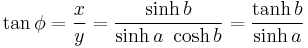$\tan \phi = \frac{x}{y} = \frac{\sinh b}{\sinh a ~\cosh b} = \frac{\tanh b}{\sinh a}$ .

As b gets large, tanh b nears one. Then tan φ = 1/sinh a . This appearance of the angle of parallelism in a meridian θ inclines one to expect to see the counter- sphere unfold as the manifold S¹ × H² where H² is the hyperbolic plane .

Application to kinematics

By using the foundations given above, one can show that the mapping

$q \mapsto u^{-1}q u$

is an ordinary or hyperbolic rotation according as

$u = e^{av} ,\quad v \in I \quad \text{or}\quad u = e^{ap} ,\quad p \in J$ .

These mappings are projectivities in the inversive ring geometry of coquaternions. The collection of these mappings bears some relation to the Lorentz group since it is also composed of ordinary and hyperbolic rotations. Among the peculiarities of this approach to relativistic kinematic is the anisotropic profile, say as compared to hyperbolic quaternions.

Reluctance to use coquaternions for kinematic models may stem from the (2, 2) signature when spacetime is presumed to have signature (1, 3) or (3, 1). Nevertheless, a transparently relativistic kinematics appears when a point of the counter-sphere is used to represent an inertial frame of reference. Indeed, if $tt^* = -1$ , then there is a p = i sinh(a) + r cosh(a) ∈ J such that t ∈ D_p, and an b ∈ R such that t = p exp(bp). Then if u = exp(bp), v = i cosh(a) + r sinh(a), and s = ir, the set {t, u, v, s} is a pan-orthogonal basis stemming from t, and the orthogonalities persist through applications of the ordinary or hyperbolic rotations.

Historical notes

The coquaternions were initially introduced (under that name) in 1849 by James Cockle in the London–Edinburgh–Dublin Philosophical Magazine (Cockle 1849). The introductory papers by Cockle were recalled in the 1904 Bibliography of the Quaternion Society. Alexander Macfarlane called the structure of coquaternion vectors an exspherical system when he was speaking at the International Congress of Mathematicians in Paris in 1900.

The unit sphere was considered in 1910 by Hans Beck (Beck 1910: e.g., the dihedral group appears on page 419). The coquaternion structure has also been mentioned briefly in the Annals of Mathematics (Albert 1942, Bargmann 1947).

Synonyms

Para-quaternions (Ivanov and Zamkovoy 2005, Mohaupt 2006) Manifolds with para-quaternionic structures are studied in differential geometry and string theory. In the para-quaternionic literature k is replaced with −k.
Musean hyperbolic quaternions
Exspherical system (Macfarlane 1900)
Split-quaternions (Rosenfeld 1988)
Antiquaternions (Rosenfeld 1988)
Pseudoquaternions (Rosenfeld 1988)

References

Albert, A.A. (1942), "Quadratic Forms permitting Composition", Annals of Mathematics 43, pp. 161–177.
Bargmann, V. (1947), "Representations of the Lorentz Group", Annals of Mathematics 48, pp. 568–640.
Beck, Hans (1910), in Transactions of the American Mathematical Society 28.
Cockle, James (1849), "On Systems of Algebra involving more than one Imaginary", Philosophical Magazine (series 3) 35, pp. 434–435.
Ivanov, Stefan; Zamkovoy, Simeon (2005), "Parahermitian and paraquaternionic manifolds", Differential Geometry and its Applications 23, pp. 205–234, math.DG/0310415 MR 2006d:53025.
Karzel, Helmut & Günter Kist (1985) "Kinematic Algebras and their Geometries", in Rings and Geometry, R. Kaya, P. Plaumann, and K. Strambach editors, pp 437–509, esp 449,50, D. Reidel ISBN 90-277-2112-2 .
Macfarlane, Alexander (1900) Proceedings of the International Congress of Mathematicians, Paris, page 306.
Macfarlane, Alexander (1904) Bibliography of Quaternions and Allied Systems of Mathematics,entries for James Cockle, pp. 17–18.
Mohaupt, Thomas (2006), "New developments in special geometry", hep-th/0602171.
Özdemir, M. (2009) "The roots of a split quaternion", Applied Mathematics Letters 22:258–63.
Özdemir, M. & A.A. Ergin (2006) "Rotations with timelike quaternions in Minkowski 3-space", Journal of Geometry and Physics 56: 322–36.
Pogoruy, Anatoliy & Ramon M Rodrigues-Dagnino (2008) Some algebraic and analytical properties of coquaternion algebra, Advances in Applied Clifford Algebras.
Rosenfeld, B.A. (1988) A History of Non-Euclidean Geometry, page 389, Springer-Verlag ISBN 0-387-96458-4 .

Number systems

Countable sets	Natural numbers ( $\scriptstyle\mathbb{N}$ ) Integers ( $\scriptstyle\mathbb{Z}$ ) Rational numbers ( $\scriptstyle\mathbb{Q}$ ) Algebraic numbers ( $\scriptstyle\overline{\mathbb{Q}}$ ) Periods Computable numbers Arithmetical numbers

Real numbers and their extensions	Real numbers ( $\scriptstyle\mathbb{R}$ ) Complex numbers ( $\scriptstyle\mathbb{C}$ ) Quaternions ( $\scriptstyle\mathbb{H}$ ) Octonions ( $\scriptstyle\mathbb{O}$ ) Sedenions ( $\scriptstyle\mathbb{S}$ ) Cayley–Dickson construction Dual numbers Hypercomplex numbers Superreal numbers Irrational numbers Transcendental numbers Hyperreal numbers Surreal numbers

Other number systems	Cardinal numbers Ordinal numbers p-adic numbers Supernatural numbers