Schwarzschild geodesics

In general relativity, the geodesics of the Schwarzschild metric describe the motion of particles of infinitesimal mass in the gravitational field of a central fixed mass M. The Schwarzschild geodesics have been pivotal in the validation of the Einstein's theory of general relativity. For example, they provide quantitative predictions of the anomalous precession of the planets in the Solar System, and of the deflection of light by gravity.

The Schwarzschild geodesics pertain only to the motion of particles of infinitesimal mass m, i.e., particles that do not themselves contribute to the gravitational field. However, they are highly accurate provided that m is many-fold smaller than the central mass M, e.g., for planets orbiting their sun. The Schwarzschild geodesics are also a good approximation to the relative motion of two bodies of arbitrary mass, provided that the Schwarzschild mass M is set equal to the sum of the two individual masses m₁ and m₂. This is important in predicting the motion of binary stars in general relativity.

Historical context

The Schwarzschild solution was found by Karl Schwarzschild shortly after Einstein published his field equations. The Schwarzschild metric is named in honour of its discoverer Karl Schwarzschild, who found the solution in 1915, only about a month after the publication of Einstein's theory of general relativity. It was the first solution of the Einstein field equations other than the trivial flat space solution.

Schwarzschild metric

An exact solution to the Einstein field equations is the Schwarzschild metric, which corresponds to the external gravitational field of an uncharged, non-rotating, spherically symmetric body of mass M. The Schwarzschild solution can be written as^[1]

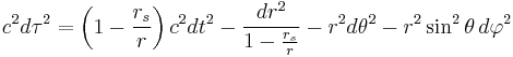
$c^2 {d \tau}^{2} = \left( 1 - \frac{r_{s}}{r} \right) c^{2} dt^{2} - \frac{dr^{2}}{1 - \frac{r_{s}}{r}} - r^{2} d\theta^{2} - r^{2} \sin^{2} \theta \, d\varphi^{2}$

where

τ is the proper time (time measured by a clock moving with the particle) in seconds,

c is the speed of light in meters per second,

t is the time coordinate (measured by a stationary clock at infinity) in seconds,

r is the radial coordinate (circumference of a circle centered on the star divided by 2π) in meters,

θ is the colatitude (angle from North) in radians,

φ is the longitude in radians, and

r_s is the Schwarzschild radius (in meters) of the massive body, which is related to its mass M by

$r_{s} = \frac{2GM}{c^{2}}$

where G is the gravitational constant. The classical Newtonian theory of gravity is recovered in the limit as the ratio r_s/r goes to zero. In that limit, the metric returns to that defined by special relativity.

In practice, this ratio is almost always extremely small. For example, the Schwarzschild radius r_s of the Earth is roughly 9 mm (³⁄₈ inch); at the surface of the Earth, the corrections to Newtonian gravity are only one part in a billion. The Schwarzschild radius of the Sun is much larger, roughly 2953 meters, but at its surface, the ratio r_s/r is roughly 4 parts in a million. A white dwarf star is much denser, but even here the ratio at its surface is roughly 250 parts in a million. The ratio only becomes large close to ultra-dense objects such as neutron stars (where the ratio is roughly 50%) and black holes.

Orbits of test particles

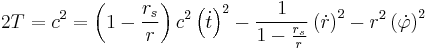
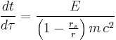
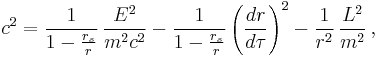
Dividing both sides by dτ², the Schwarzschild metric can be rewritten as

$c^{2} = \left( 1 - \frac{r_{s}}{r} \right) c^{2} \left( \frac{dt}{d\tau} \right)^{2} - \frac{1}{1 - \frac{r_{s}}{r}} \left( \frac{dr}{d\tau} \right)^{2} - r^{2} \left( \frac{d\theta}{d\tau} \right)^{2} - r^{2} \sin^{2} \theta \, \left( \frac{d\varphi}{d\tau} \right)^{2},$

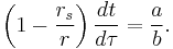
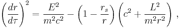
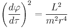
The orbit of a particle in this metric is defined by the geodesic equation, which may be solved by any of several methods (as outlined below). This equation yields three constants of motion. First, the motion of the particle is always in a plane, which is equivalent to fixing θ = π/2. The second and third constants of motion, derived below, are taken as two length-scales, a and b, defined by the equations

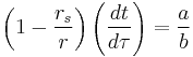
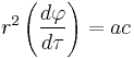
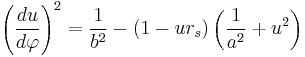
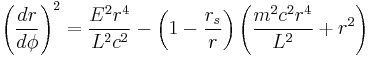
$\left( 1 - \frac{r_{s}}{r} \right) \left( \frac{dt}{d\tau} \right) = \frac{a}{b}$

$r^{2} \left( \frac{d\varphi}{d\tau} \right) = a c$

where c represents the speed of light. Incorporating these constants of motion into the metric yields the fundamental equation for the particle's orbit

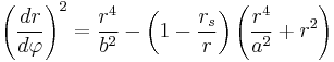
$\left( \frac{dr}{d\varphi} \right)^{2} = \frac{r^{4}}{b^{2}} - \left( 1 - \frac{r_{s}}{r} \right) \left( \frac{r^{4}}{a^{2}} %2B r^{2} \right)$

Exact solution using elliptic functions

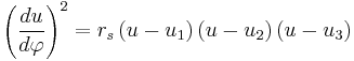
The fundamental equation of the orbit is easier to solve^{[note 1]} if it is expressed in terms of the inverse radius u = 1/r

$\left( \frac{du}{d\varphi} \right)^{2} = \frac{1}{b^{2}} - \left( 1 - u r_{s} \right) \left( \frac{1}{a^{2}} %2B u^{2} \right)$

The right-hand side of this equation is a cubic polynomial, which has three roots, denoted here as u₁, u₂, and u₃

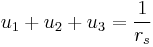
$\left( \frac{du}{d\varphi} \right)^{2} = r_{s} \left( u - u_{1} \right) \left( u - u_{2} \right) \left( u - u_{3} \right)$

The sum of the three roots equals the coefficient of the u² term

$u_{1} %2B u_{2} %2B u_{3} = \frac{1}{r_{s}}$

A cubic polynomial with real coefficients can either have three real roots, or one real root and two complex conjugate roots. If all three roots are real numbers, the roots are labeled so that u₁ < u₂ < u₃. If instead there is only one real root, then that is denoted as u₃; the complex conjugate roots are labeled u₁ and u₂. Using Descartes' rule of signs, there can be at most one negative root; u₁ is negative if and only if b < a. As discussed below, the roots are useful in determining the types of possible orbits.

Given this labeling of the roots, the solution of the fundamental orbital equation for the orbit can be expressed in elliptic functions

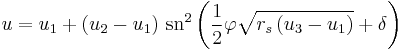
$u = u_{1} %2B \left( u_{2} - u_{1} \right) \, \mathrm{sn}^{2}\left( \frac{1}{2} \varphi \sqrt{r_{s} \left( u_{3} - u_{1} \right)} %2B \delta \right)$

where sn represents one of the Jacobi elliptic functions and δ is a constant of integration reflecting the initial position. The modulus k of this elliptic function is given by the formula

$k = \sqrt{\frac{u_{2} - u_{1}}{u_{3} - u_{1}}}$

Classical limit

To recover the Newtonian solution for the planetary orbits, one takes the limit as the Schwarzschild radius r_s goes to zero. In this case, the third root u₃ becomes roughly 1/r_s, and much larger than u₁ or u₂. Therefore, the modulus k tends to zero; in that limit, sn becomes the trigonometric sine function

$u = u_{1} %2B \left( u_{2} - u_{1} \right) \, \sin^{2}\left( \frac{1}{2} \varphi %2B \delta \right)$

Consistent with Newton's solutions for planetary motions, this formula describes a focal conic of eccentricity e

$e = \frac{u_{2} - u_{1}}{u_{2} %2B u_{1}}$

If u₁ is a positive real number, then the orbit is an ellipse where u₁ and u₂ represent the distances of furthest and closest approach, respectively. If u₁ is zero or a negative real number, the orbit is a parabola or a hyperbola, respectively. In these latter two cases, u₂ represents the distance of closest approach; since the orbit goes to infinity (u=0), there is no distance of furthest approach.

Roots and overview of possible orbits

A root represents a point of the orbit where the derivative vanishes, i.e., where du/dφ = 0. At such a turning point, u reaches a maximum, a minimum, or an inflection point, depending on the value of the second derivative, which is given by the formula

$\frac{d^{2}u}{d\varphi^{2}} = \frac{r_{s}}{2} \left[ \left( u - u_{2} \right) \left( u - u_{3} \right) %2B \left( u - u_{1} \right) \left( u - u_{3} \right) %2B \left( u - u_{1} \right) \left( u - u_{2} \right) \right]$

Therefore, if all three roots are distinct real numbers, the second derivative is positive, negative, and positive at u₁,u₂, and u₃, respectively. It follows that the system may either oscillate between u₁ and u₂, or it may move away from u₃ towards infinity. Circular orbits result if u₂ is equal to either u₁ or u₃. These different types of orbits are discussed in the following subsections.

Precession of orbits

The function sn and its square sn² have periods of 4K and 2K, respectively, where K is defined by the equation^{[note 2]}

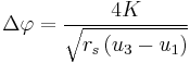
$K = \int_{0}^{1} \frac{dy}{\sqrt{\left( 1 - y^{2} \right) \left( 1 - k^{2} y^{2} \right) }}$

Therefore, the change in φ over one oscillation of u (or, equivalently, one oscillation of r) equals^[2]

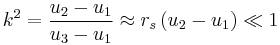
$\Delta \varphi = \frac{4K}{\sqrt{r_{s} \left( u_{3} - u_{1} \right) }}$

In the classical limit, u₃ approaches 1/r_s and is much larger than u₁ or u₂. Hence, k² is approximately

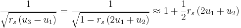
$k^{2} = \frac{u_{2} - u_{1}}{u_{3} - u_{1}} \approx r_{s} \left( u_{2} - u_{1} \right) \ll 1$

For the same reasons, the denominator of Δφ is approximately

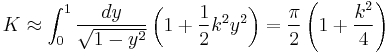
$\frac{1}{\sqrt{r_{s} \left( u_{3} - u_{1} \right) }} = \frac{1}{\sqrt{1 - r_{s} \left(2 u_{1} %2B u_{2} \right)}} \approx 1 %2B \frac{1}{2} r_{s} \left( 2u_{1} %2B u_{2} \right)$

Since the modulus k is close to zero, the period K can be expanded in powers of k; to lowest order, this expansion yields

$K \approx \int_{0}^{1} \frac{dy}{\sqrt{1 - y^{2} }} \left( 1 %2B \frac{1}{2} k^{2} y^{2} \right) = \frac{\pi}{2} \left( 1 %2B \frac{k^{2}}{4} \right)$

Substituting these approximations into the formula for Δφ yields a formula for angular advance per radial oscillation

$\delta \varphi = \Delta \varphi - 2\pi \approx \frac{3}{2} \pi r_{s} \left( u_{1} %2B u_{2} \right)$

For an elliptical orbit, u₁ and u₂ represent the inverses of the longest and shortest distances, respectively. These can be expressed in terms of the ellipse's semiaxis A and its eccentricity e,

$r_{\mathrm{max}} = \frac{1}{u_{1}} = A (1 %2B e)$

$r_{\mathrm{min}} = \frac{1}{u_{2}} = A (1 - e)$

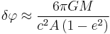
giving

$u_{1} %2B u_{2} = \frac{1}{A \left( 1 - e^{2} \right)}$

Substituting the definition of r_s gives the final equation

$\delta \varphi \approx \frac{6\pi G M}{c^{2} A \left( 1 - e^{2} \right)}$

Bending of light by gravity

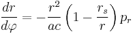
See also: Gravitational lens and Shapiro delay

In the limit as the particle mass m goes to zero (or, equivalently, as the length-scale a goes to infinity), the equation for the orbit becomes

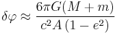
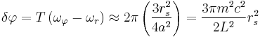
$\varphi = \int \frac{dr}{r^{2} \sqrt{\frac{1}{b^{2}} - \left( 1 - \frac{r_{s}}{r} \right) \frac{1}{r^{2}}}}$

Expanding in powers of r_s/r, the leading order term in this formula gives the approximate angular deflection δφ for a massless particle coming in from infinity and going back out to infinity:

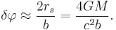
$\delta \varphi \approx \frac{2r_{s}}{b} = \frac{4GM}{c^{2}b}.$

Here, b can be interpreted as the distance of closest approach. Although this formula is approximate, it is accurate for most measurements of gravitational lensing, due to the smallness of the ratio r_s/r. For light grazing the surface of the sun, the approximate angular deflection is roughly 1.75 arcseconds, roughly one millionth part of a circle.

Relation to classical physics

Effective radial potential energy

The equation of motion for the particle derived above

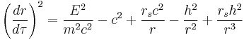
$\left( \frac{dr}{d\tau} \right)^{2} = \frac{E^2}{m^2 c^2} - c^{2} %2B \frac{ r_{s} c^2}{r} - \frac{h^2}{ r^2 } %2B \frac{ r_{s} h^2 }{ r^3 }$

can be rewritten using the definition of the Schwarzschild radius r_s as

$\frac{1}{2} m \left( \frac{dr}{d\tau} \right)^{2} = \left[ \frac{E^2}{2 m c^2} - \frac{1}{2} m c^2 \right] %2B \frac{GMm}{r} - \frac{ L^2 }{ 2 \mu r^2 } %2B \frac{ G(M%2Bm) L^2 }{c^2 \mu r^3}$

which is equivalent to a particle moving in a one-dimensional effective potential

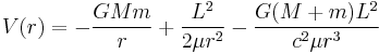
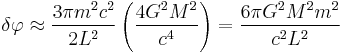
$V(r) = -\frac{GMm}{r} %2B \frac{ L^2 }{ 2 \mu r^2 } - \frac{ G(M%2Bm) L^2 }{ c^2 \mu r^3 }$

The first two terms are well-known classical energies, the first being the attractive Newtonian gravitational potential energy and the second corresponding to the repulsive "centrifugal" potential energy; however, the third term is an attractive energy unique to general relativity. As shown below and elsewhere, this inverse-cubic energy causes elliptical orbits to precess gradually by an angle δφ per revolution

$\delta \varphi \approx \frac{ 6\pi G(M%2Bm) }{ c^2 A \left( 1- e^{2} \right)}$

where A is the semi-major axis and e is the eccentricity.

The third term is attractive and dominates at small r values, giving a critical inner radius r_inner at which a particle is drawn inexorably inwards to r=0; this inner radius is a function of the particle's angular momentum per unit mass or, equivalently, the a length-scale defined above.

Circular orbits and their stability

The effective potential V can be re-written in terms of the lengths a and b

$V(r) = \frac{mc^{2}}{2} \left[ - \frac{r_{s}}{r} %2B \frac{a^{2}}{r^{2}} - \frac{r_{s} a^{2}}{r^{3}} \right]$

Circular orbits are possible when the effective force is zero

$F = -\frac{dV}{dr} = -\frac{mc^{2}}{2r^{4}} \left[ r_{s} r^{2} - 2a^{2} r %2B 3r_{s} a^{2} \right] = 0$

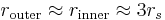
i.e., when the two attractive forces — Newtonian gravity (first term) and the attraction unique to general relativity (third term) — are exactly balanced by the repulsive centrifugal force (second term). There are two radii at which this balancing can occur, denoted here as r_inner and r_outer

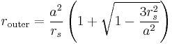
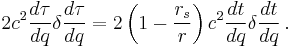
$r_{\mathrm{outer}} = \frac{a^{2}}{r_{s}} \left( 1 %2B \sqrt{1 - \frac{3r_{s}^{2}}{a^{2}}} \right)$

$r_{\mathrm{inner}} = \frac{a^{2}}{r_{s}} \left( 1 - \sqrt{1 - \frac{3r_{s}^{2}}{a^{2}}} \right) = \frac{3a^{2}}{r_{\mathrm{outer}}}$

which are obtained using the quadratic formula. The inner radiusr_inner is unstable, because the attractive third force strengthens much faster than the other two forces whenr becomes small; if the particle slips slightly inwards from r_inner (where all three forces are in balance), the third force dominates the other two and draws the particle inexorably inwards to r=0. At the outer radius, however, the circular orbits are stable; the third term is less important and the system behaves more like the non-relativistic Kepler problem.

When a is much greater than r_s (the classical case), these formulae become approximately

$r_{\mathrm{outer}} \approx \frac{2a^{2}}{r_{s}}$

$r_{\mathrm{inner}} \approx \frac{3}{2} r_{s}$

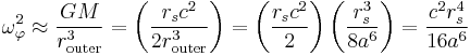
Substituting the definitions of a and r_s into r_outer yields the classical formula for a particle orbiting a mass M in a circle

$r_{\mathrm{outer}}^{3} \approx \frac{GM}{\omega_{\varphi}^{2}}$

where ω_φ is the orbital angular speed of the particle. This formula is obtained in non-relativistic mechanics by setting the centrifugal force equal to the Newtonian gravitational force:

$\frac{GMm}{r^{2}} = \mu \omega_{\varphi}^{2} r$

Where $\mu$ is the reduced mass.
In our notation, the classical orbital angular speed equals

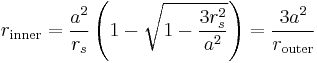
$\omega_{\varphi}^{2} \approx \frac{GM}{r_{\mathrm{outer}}^{3}} = \left( \frac{r_{s} c^{2}}{2r_{\mathrm{outer}}^{3}} \right) = \left( \frac{r_{s} c^{2}}{2} \right) \left( \frac{r_{s}^{3}}{8a^{6}}\right) = \frac{c^{2} r_{s}^{4}}{16 a^{6}}$

At the other extreme, when a² approaches 3r_s² from above, the two radii converge to a single value

$r_{\mathrm{outer}} \approx r_{\mathrm{inner}} \approx 3 r_{s}$

The quadratic solutions above ensure that r_outer is always greater than 3r_s, whereas r_inner lies between ³⁄₂ r_s and 3r_s. Circular orbits smaller than ³⁄₂ r_s are not possible. For massless particles, a goes to infinity, implying that there is a circular orbit for photons at r_inner =³⁄₂ r_s. The sphere of this radius is sometimes known as the photon sphere.

Precession of elliptical orbits

The orbital precession rate may be derived using this radial effective potential V. A small radial deviation from a circular orbit of radius r_outer will oscillate stably with an angular frequency

$\omega_{r}^{2} = \frac{1}{m} \left[ \frac{d^{2}V}{dr^{2}} \right]_{r=r_{\mathrm{outer}}}$

which equals

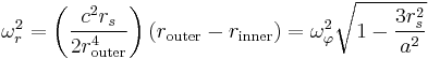
$\omega_{r}^{2} = \left( \frac{c^{2} r_{s}}{2 r_{\mathrm{outer}}^{4}} \right) \left( r_{\mathrm{outer}} - r_{\mathrm{inner}}\right) = \omega_{\varphi}^{2} \sqrt{1 - \frac{3r_{s}^{2}}{a^{2}}}$

Taking the square root of both sides and expanding using the binomial theorem yields the formula

$\omega_{r} = \omega_{\varphi} \left( 1 - \frac{3r_{s}^{2}}{4a^{2}} %2B \cdots \right)$

Multiplying by the period T of one revolution gives the precession of the orbit per revolution

$\delta \varphi = T \left( \omega_{\varphi} - \omega_{r} \right) \approx 2\pi \left( \frac{3r_{s}^{2}}{4a^{2}} \right) = \frac{3\pi m^{2} c^{2}}{2L^{2}} r_{s}^{2}$

where we have used ω_φT = 2п and the definition of the length-scale a. Substituting the definition of the Schwarzschild radius r_s gives

$\delta \varphi \approx \frac{3\pi m^{2} c^{2}}{2L^{2}} \left( \frac{4G^{2} M^{2}}{c^{4}} \right) = \frac{6\pi G^{2} M^{2} m^{2}}{c^{2} L^{2}}$

This may be simplified using the elliptical orbit's semiaxis A and eccentricity e related by the formula

$\frac{ h^2 }{ G(M%2Bm) } = A \left( 1 - e^2 \right)$

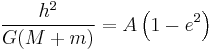
to give the precession angle

$\delta \varphi \approx \frac{6\pi G(M%2Bm)}{c^2 A \left( 1 - e^{2} \right)}$

Mathematical derivations of the orbital equation

Geodesic equation

According to Einstein's theory of general relativity, particles of negligible mass travel along geodesics in the space-time. In uncurved (flat) space-time, far from a source of gravity, these geodesics correspond to straight lines; however, they may deviate from straight lines when the space-time is curved. The equation for the geodesic lines is^[3]

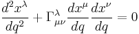
$\frac{d^2x^{\lambda}}{d q^2} %2B \Gamma^{\lambda}_{\mu\nu} \frac{dx^{\mu}}{d q} \frac{dx^{\nu}}{dq} = 0$

where Γ represents the Christoffel symbol and the variable q parametrizes the particle's path through space-time, its so-called world line. The Christoffel symbol depends only on the metric tensor g_μν, or rather on how it changes with position. The variable q is a constant multiple of the proper time τ for timelike orbits (which are traveled by massive particles), and is usually taken to be equal to it. For lightlike (or null) orbits (which are traveled by massless particles such as the photon), the proper time is zero and, strictly speaking, cannot be used as the variable q. Nevertheless, lightlike orbits can be derived as the ultrarelativistic limit of timelike orbits, that is, the limit as the particle mass m goes to zero while holding its total energy fixed.

Therefore, to solve for the motion of a particle, the most straightforward way is to solve the geodesic equation, an approach adopted by Einstein^[4] and others.^[5] The Schwarzschild metric may be written as

$c^{2}d\tau^{2} = w(r) c^2 dt^{2} - v(r) dr^{2} - r^{2} d\theta^{2} - r^{2} \sin^{2} \theta d\phi^{2} \,$

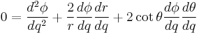
where the two functions w(r) = (1 - r_s/r) and its inverse v(r) = 1/w(r) are be defined for brevity. From this metric, the Christoffel symbols Γ^λ_μν may be calculated, and the results substituted into the geodesic equations

$0 = \frac{d^{2}\theta}{dq^{2}} %2B \frac{2}{r} \frac{d\theta}{dq} \frac{dr}{dq} - \sin \theta \cos \theta \left( \frac{d\phi}{dq} \right)^{2}$

$0 = \frac{d^{2}\phi}{dq^{2}} %2B \frac{2}{r} \frac{d\phi}{dq} \frac{dr}{dq} %2B 2 \cot \theta \frac{d\phi}{dq} \frac{d\theta}{dq}$

$0 = \frac{d^{2}t}{dq^{2}} %2B \frac{1}{w} \frac{dw}{dr} \frac{dt}{dq} \frac{dr}{dq}$

$0 = \frac{d^{2}r}{dq^{2}} %2B \frac{1}{2v} \frac{dv}{dr} \left( \frac{dr}{dq} \right)^{2} - \frac{r}{v} \left( \frac{d\theta}{dq} \right)^{2} - \frac{r\sin^{2}\theta}{v} \left( \frac{d\phi}{dq} \right)^{2} %2B \frac{c^{2}}{2v} \frac{dw}{dr} \left( \frac{dt}{dq} \right)^{2}$

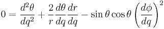
It may be verified that θ=π/2 is a valid solution by substitution into the first of these four equations. By symmetry, the orbit must be planar, and we are free to arrange the coordinate frame so that the equatorial plane is the plane of the orbit. This θ solution simplifies the second and fourth equations.

To solve the second and third equations, it suffices to divide them by dφ/dq and dt/dq, respectively.

$0 = \frac{d}{dq} \left[ \ln \frac{d\phi}{dq} %2B \ln r^{2} \right]$

$0 = \frac{d}{dq} \left[ \ln \frac{dt}{dq} %2B \ln w \right]$

which yields two constants of motion.

Lagrangian approach

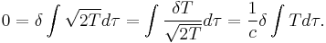
Because test particles follow geodesics in a fixed metric, the orbits of those particles may be determined using the calculus of variations, also called the Lagrangian approach.^[6] Geodesics in space-time are defined as curves for which small local variations in their coordinates (while holding their endpoints events fixed) make no significant change in their overall length s. This may be expressed mathematically using the calculus of variations

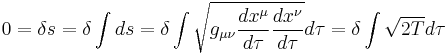
$0 = \delta s = \delta \int ds = \delta \int \sqrt{g_{\mu\nu} \frac{dx^{\mu}}{d\tau} \frac{dx^{\nu}}{d\tau} } d\tau = \delta \int \sqrt{2T} d\tau$

where τ is the proper time, s=cτ is the arc-length in space-time and T is defined as

$2T = c^{2} = \left( \frac{ds}{d\tau} \right)^{2} = g_{\mu\nu} \frac{dx^{\mu}}{d\tau} \frac{dx^{\nu}}{d\tau} = \left( 1 - \frac{r_{s}}{r} \right) c^{2} \left( \frac{dt}{d\tau} \right)^{2} - \frac{1}{1 - \frac{r_{s}}{r}} \left( \frac{dr}{d\tau} \right)^{2} - r^{2} \left( \frac{d\varphi}{d\tau} \right)^{2}$

in analogy with kinetic energy. If the derivative with respect to proper time is represented by a dot for brevity

$\dot{x}^{\mu} = \frac{dx^{\mu}}{d\tau}$

T may be written as

$2T = c^{2} = \left( 1 - \frac{r_{s}}{r} \right) c^{2} \left( \dot{t} \right)^{2} - \frac{1}{1 - \frac{r_{s}}{r}} \left( \dot{r} \right)^{2} - r^{2} \left( \dot{\varphi} \right)^{2}$

Constant factors (such as c or the square root of two) don't affect the answer to the variational problem; therefore, taking the variation inside the integral yields Hamilton's principle

$0 = \delta \int \sqrt{2T} d\tau = \int \frac{\delta T}{\sqrt{2T}} d\tau = \frac{1}{c} \delta \int T d\tau.$

The solution of the variational problem is given by Lagrange's equations

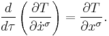
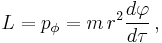
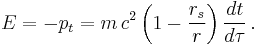
$\frac{d}{d\tau} \left(\frac{\partial T}{\partial \dot{x}^{\sigma}} \right) = \frac{\partial T}{\partial x^{\sigma}}.$

When applied to t and φ, these equations reveal two constants of motion

$\frac{d}{d\tau} \left[ r^{2} \frac{d\varphi}{d\tau} \right] = 0,$

$\frac{d}{d\tau} \left[ \left( 1 - \frac{r_{s}}{r} \right) \frac{dt}{d\tau} \right] = 0,$

which may be expressed in terms of two constant length-scales, a and b

$r^{2} \frac{d\varphi}{d\tau} = ac,$

$\left( 1 - \frac{r_{s}}{r} \right) \frac{dt}{d\tau} = \frac{a}{b}.$

As shown above, substitution of these equations into the definition of the Schwarzschild metric yields the equation for the orbit.

Hamiltonian approach

A Lagrangian solution can be recast into an equivalent Hamiltonian form.^[7] In this case, the Hamiltonian H is given by

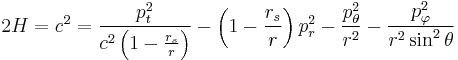
$2 H = c^{2} = \frac{p_{t}^{2}}{c^{2} \left( 1 - \frac{r_{s}}{r} \right)} - \left( 1 - \frac{r_{s}}{r} \right) p_{r}^{2} - \frac{p_{\theta}^{2}}{r^{2}} - \frac{p_{\varphi}^{2}}{r^{2}\sin^{2} \theta}$

Once again, the orbit may be restricted to θ = π/2 by symmetry. Since t, θ and φ do not appear in the Hamiltonian, their conjugate momenta are constant; they may be expressed in terms of the speed of light c and two constant length-scales a and b

$p_{\varphi} = - ac$

$p_{\theta} = 0$

$p_{t} = \frac{ac^{2}}{b}$

The derivatives with respect to proper time are given by

$\frac{dr}{d\tau} = \frac{\partial H}{\partial p_{r}} = - \left(1 - \frac{r_{s}}{r} \right) p_{r}$

$\frac{d\varphi}{d\tau} = \frac{\partial H}{\partial p_{\varphi}} = \frac{-p_{\varphi}}{r^{2}} = \frac{ac}{r^{2}}$

$\frac{dt}{d\tau} = \frac{\partial H}{\partial p_{t}} = \frac{p_{t}}{c^{2} \left( 1 - \frac{r_{s}}{r} \right)} = \frac{a}{b \left( 1 - \frac{r_{s}}{r} \right)}$

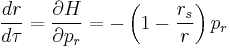
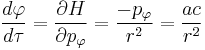
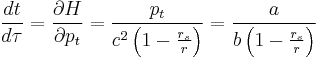
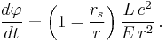
Dividing the first equation by the second yields the orbital equation

$\frac{dr}{d\varphi} = - \frac{r^{2}}{ac} \left(1 - \frac{r_{s}}{r} \right) p_{r}$

The radial momentum p_r can be expressed in terms of r using the constancy of the Hamiltonian H = c²/2; this yields the fundamental orbital equation

$\left( \frac{dr}{d\varphi} \right)^{2} = \frac{r^{4}}{b^{2}} - \left( 1 - \frac{r_{s}}{r} \right) \left( \frac{r^{4}}{a^{2}} %2B r^{2} \right)$

Hamilton–Jacobi approach

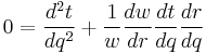
The orbital equation can be derived from the Hamilton–Jacobi equation.^[8] The advantage of this approach is that it equates the motion of the particle with the propagation of a wave, and leads neatly into the derivation of the deflection of light by gravity in general relativity, through Fermat's principle. The basic idea is that, due to gravitational slowing of time, parts of a wave-front closer to a gravitating mass move more slowly than those further away, thus bending the direction of the wave-front's propagation.

Using general covariance, the Hamilton–Jacobi equation for a single particle of unit mass can be expressed in arbitrary coordinates as

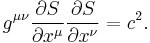
$g^{\mu\nu} \frac{\partial S}{\partial x^{\mu}} \frac{\partial S}{\partial x^{\nu}} = c^{2}.$

This is equivalent to the Hamiltonian formulation above, with the partial derivatives of the action taking the place of the generalized momenta. Using the Schwarzschild metric g^μν, this equation becomes

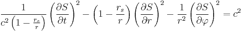
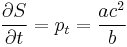
$\frac{1}{c^{2} \left(1 - \frac{r_{s}}{r} \right)} \left( \frac{\partial S}{\partial t} \right)^{2} - \left( 1 - \frac{r_{s}}{r} \right) \left( \frac{\partial S}{\partial r} \right)^{2} - \frac{1}{r^{2}} \left( \frac{\partial S}{\partial \varphi} \right)^{2} = c^{2}$

where we again orient the spherical coordinate system with the plane of the orbit. The time t and azimuthal angle φ are cyclic coordinates, so that the solution for Hamilton's principal function S can be written

$S = -p_{t} t %2B p_{\varphi} \varphi %2B S_{r}(r) \,$

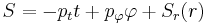
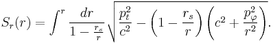
where p_t and p_φ are the constant generalized momenta. The Hamilton–Jacobi equation gives an integral solution for the radial part S_r(r)

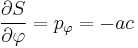
$S_{r}(r) = \int^{r} \frac{dr}{1 - \frac{r_{s}}{r}} \sqrt{\frac{p_{t}^{2}}{c^{2}} - \left( 1 - \frac{r_{s}}{r} \right) \left( c^{2} %2B \frac{p_{\varphi}^{2}}{r^{2}} \right)}.$

Taking the derivative of Hamilton's principal function S with respect to the conserved momentum p_φ yields

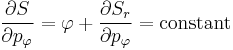
$\frac{\partial S}{\partial p_{\varphi}} = \varphi %2B \frac{\partial S_{r}}{\partial p_{\varphi}} = \mathrm{constant}$

which equals

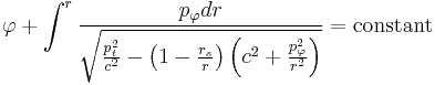
$\varphi %2B \int^{r} \frac{p_{\varphi} dr}{\sqrt{\frac{p_{t}^{2}}{c^{2}} - \left( 1 - \frac{r_{s}}{r} \right) \left( c^{2} %2B \frac{p_{\varphi}^{2}}{r^{2}} \right)}} = \mathrm{constant}$

Taking an infinitesimal variation in φ and r yields the fundamental orbital equation

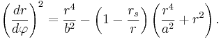
$\left( \frac{dr}{d\varphi} \right)^{2} = \frac{r^{4}}{b^{2}} - \left( 1 - \frac{r_{s}}{r} \right) \left( \frac{r^{4}}{a^{2}} %2B r^{2} \right).$

where the conserved length-scales a and b are defined by the conserved momenta by the equations

$\frac{\partial S}{\partial \varphi} = p_{\varphi} = -ac$

$\frac{\partial S}{\partial t} = p_{t} = \frac{ac^{2}}{b}$

Hamilton's principle

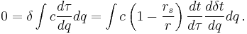
The action integral for a particle affected only by gravity is

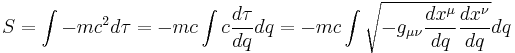
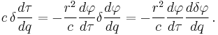
$S = \int{ - m c^2 d\tau} = - m c \int{ c \frac{d\tau}{dq} dq} = - m c \int{ \sqrt{-g_{\mu\nu} \frac{dx^{\mu}}{dq} \frac{dx^{\nu}}{dq} } dq}$

where τ is the proper time and q is any smooth parameterization of the particle's world line. If one applies the calculus of variations to this, one again gets the equations for a geodesic. To simplify the calculations, one first takes the variation of the square of the integrand. For the metric and coordinates of this case and assuming that the particle is moving in the equatorial plane (θ= π/2), that square is

$\left(c \frac{d\tau}{dq}\right)^2 = - g_{\mu\nu} \frac{dx^{\mu}}{dq} \frac{dx^{\nu}}{dq} = \left( 1 - \frac{r_{s}}{r} \right) c^{2} \left( \frac{dt}{dq} \right)^{2} - \frac{1}{1 - \frac{r_{s}}{r}} \left( \frac{dr}{dq} \right)^{2} - r^{2} \left( \frac{d\varphi}{dq} \right)^{2} \,.$

Taking variation of this gives

$\delta \left(c \frac{d\tau}{dq}\right)^2 = 2 c^{2} \frac{d\tau}{dq} \delta \frac{d\tau}{dq} = \delta \left[ \left( 1 - \frac{r_{s}}{r} \right) c^{2} \left( \frac{dt}{dq} \right)^{2} - \frac{1}{1 - \frac{r_{s}}{r}} \left( \frac{dr}{dq} \right)^{2} - r^{2} \left( \frac{d\varphi}{dq} \right)^{2} \right] \,.$

Motion in longitude

Vary with respect to longitude φ only to get

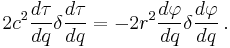
$2 c^{2} \frac{d\tau}{dq} \delta \frac{d\tau}{dq} = - 2 r^{2} \frac{d\varphi}{dq} \delta \frac{d\varphi}{dq} \,.$

Divide by $2 c \frac{d\tau}{dq}$ to get the variation of the integrand itself

$c \, \delta \frac{d\tau}{dq} = - \frac{r^{2}}{c} \frac{d\varphi}{d\tau} \delta \frac{d\varphi}{dq} = - \frac{r^{2}}{c} \frac{d\varphi}{d\tau} \frac{d \delta \varphi}{dq} \,.$

Thus

$0 = \delta \int { c \frac{d\tau}{dq} dq } = \int { c \delta \frac{d\tau}{dq} dq } = \int { - \frac{r^{2}}{c} \frac{d\varphi}{d\tau} \frac{d \delta \varphi}{dq} dq } \,.$

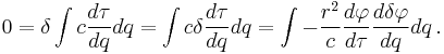
Integrating by parts gives

$0 = - \frac{r^{2}}{c} \frac{d\varphi}{d\tau} \delta \varphi - \int { \frac{d}{dq} \left[ - \frac{r^{2}}{c} \frac{d\varphi}{d\tau} \right] \delta \varphi dq } \,.$

The variation of the longitude is assumed to be zero at the end points, so the first term disappears. The integral can be made nonzero by a perverse choice of δφ unless the other factor inside is zero everywhere. So the equation of motion is

$\frac{d}{dq} \left[ - \frac{r^{2}}{c} \frac{d\varphi}{d\tau} \right] = 0 \,.$

Motion in time

Vary with respect to time t only to get

$2 c^{2} \frac{d\tau}{dq} \delta \frac{d\tau}{dq} = 2 \left( 1 - \frac{r_{s}}{r} \right) c^{2} \frac{dt}{dq} \delta \frac{dt}{dq} \,.$

Divide by $2 c \frac{d\tau}{dq}$ to get the variation of the integrand itself

$c \delta \frac{d\tau}{dq} = c \left( 1 - \frac{r_{s}}{r} \right) \frac{dt}{d\tau} \delta \frac{dt}{dq} = c \left( 1 - \frac{r_{s}}{r} \right) \frac{dt}{d\tau} \frac{d \delta t}{dq} \,.$

Thus

$0 = \delta \int { c \frac{d\tau}{dq} dq } = \int { c \left( 1 - \frac{r_{s}}{r} \right) \frac{dt}{d\tau} \frac{d \delta t}{dq} dq } \,.$

Integrating by parts gives

$0 = c \left( 1 - \frac{r_{s}}{r} \right) \frac{dt}{d\tau} \delta t - \int { \frac{d}{dq} \left[ c \left( 1 - \frac{r_{s}}{r} \right) \frac{dt}{d\tau} \right] \delta t dq } \,.$

So the equation of motion is

$\frac{d}{dq} \left[ c \left( 1 - \frac{r_{s}}{r} \right) \frac{dt}{d\tau} \right] = 0 \,.$

Conserved momenta

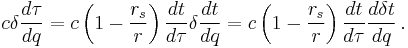
Integrate these equations of motion to determine the constants of integration getting

$L = p_{\phi} = m \, r^{2} \frac{d\varphi}{d\tau} \,,$

$E = - p_{t} = m \, c^2 \left( 1 - \frac{r_{s}}{r} \right) \frac{dt}{d\tau} \,.$

These two equations for the constants of motion L (angular momentum) and E (energy) can be combined to form one equation that is true even for photons and other massless particles for which the proper time along a geodesic is zero.

$\frac{d\varphi}{dt} = \left( 1 - \frac{r_{s}}{r} \right) \frac{L \, c^2}{E \, r^2} \,.$

Radial motion

Substituting

$\frac{d\varphi}{d\tau} = \frac{L}{m \, r^2} \,$

and

$\frac{dt}{d\tau} = \frac{E}{\left( 1 - \frac{r_{s}}{r} \right) m \, c^2} \,$

into the metric equation (and using θ=π/2) gives

$c^{2} = \frac{1}{1 - \frac{r_{s}}{r}} \, \frac{E^2}{m^2 c^2} - \frac{1}{1 - \frac{r_{s}}{r}} \left( \frac{dr}{d\tau} \right)^{2} - \frac{1}{r^{2}} \, \frac{L^2}{m^2} \,,$

from which one can derive

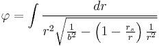
${\left( \frac{dr}{d\tau} \right)}^{2} = \frac{E^2}{m^2 c^2} - \left( 1 - \frac{r_{s}}{r} \right) \left( c^{2} %2B \frac{L^2}{m^2 r^2} \right) \,,$

which is the equation of motion for r. The dependence of r on φ can be found by dividing this by

${\left( \frac{d\varphi}{d\tau} \right)}^2 = \frac{L^2}{m^2 r^4}$

to get

${\left( \frac{dr}{d\phi} \right)}^{2} = \frac{E^2 r^4}{L^2 c^2} - \left( 1 - \frac{r_{s}}{r} \right) \left( \frac{m^2 c^{2} r^4}{L^2} %2B r^2 \right) \,$

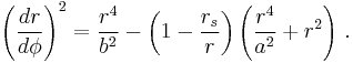
which is true even for particles without mass. If length scales are defined by

$a = \frac{L}{m \, c}$

and

$b = \frac{L \, c}{E} \,,$

then the dependence of r on φ simplifies to

${\left( \frac{dr}{d\phi} \right)}^{2} = \frac{r^4}{b^2} - \left( 1 - \frac{r_{s}}{r} \right) \left( \frac{r^4}{a^2} %2B r^2 \right) \,.$

Notes

^ This substitution of u for r is also common in classical central-force problems, since it also renders those equations easier to solve. For further information, please see the article on the classical central-force problem.
^ In the mathematical literature, K is known as the complete elliptic integral of the first kind; for further information, please see the article on elliptic integrals.

References

^ Landau and Lifshitz, pp. 299–301.
^ Synge, pp. 294–295.}
^ Weinberg, p. 122.
^ Einstein, pp. 95–96.
^ Weinberg, pp. 185–188; Wald, pp. 138–139.
^ Synge, pp. 290–292; Adler, Bazin, and Schiffer, pp. 179–182; Whittaker, pp. 390–393; Pauli, p. 167.
^ Lanczos, pp. 331–338.
^ Landau and Lifshitz, pp. 306–307; Misner, Thorne, and Wheeler, pp. 636–679.

Bibliography

Schwarzschild, K. (1916). Über das Gravitationsfeld eines Massenpunktes nach der Einstein'schen Theorie. Sitzungsberichte der Königlich Preussischen Akademie der Wissenschaften 1, 189–196.
Schwarzschild, K. (1916). Über das Gravitationsfeld einer Kugel aus inkompressibler Flüssigkeit. Sitzungsberichte der Königlich Preussischen Akademie der Wissenschaften 1, 424-?.

Flamm, L (1916). "Beiträge zur Einstein'schen Gravitationstheorie". Physikalische Zeitschrift 17: 448–?.

Adler, R; Bazin M, and Schiffer M (1965). Introduction to General Relativity. New York: McGraw-Hill Book Company. pp. 177–193. ISBN 978-0-07-000420-7.

Einstein, A (1956). The Meaning of Relativity (5th ed.). Princeton, NJ: Princeton University Press. pp. 92–97. ISBN 978-0-691-02352-6.

Hagihara, Y (1931). "Theory of the relativistic trajectories in a gravitational field of Schwarzschild". Japanese Journal of Astronomy and Geophysics 8: 67–176. ISSN 0368-346X.

Lanczos, C (1986). The Variational Principles of Mechanics (4th ed.). New York: Dover Publications. pp. 330–338. ISBN 978-0-486-65067-8.

Landau, LD; Lifshitz, EM (1975). The Classical Theory of Fields. Course of Theoretical Physics. Vol. 2 (revised 4th English ed.). New York: Pergamon Press. pp. 299–309. ISBN 978-0-08-018176-9.

Misner, CW; Thorne, K, and Wheeler, JA (1973). Gravitation. San Francisco: W. H. Freeman. pp. Chapter 25 (pp. 636–687), §33.5 (pp. 897–901), and §40.5 (pp. 1110–1116). ISBN 978-0-7167-0344-0. (See Gravitation (book).)

Pais, A. (1982). Subtle is the Lord: The Science and the Life of Albert Einstein. Oxford University Press. pp. 253–256. ISBN 0-19-520438-7.

Pauli, W (1958). Theory of Relativity. Translated by G. Field. New York: Dover Publications. pp. 40–41, 166–169. ISBN 978-0-486-64152-2.

Rindler, W (1977). Essential Relativity: Special, General, and Cosmological (revised 2nd ed.). New York: Springer Verlag. pp. 143–149. ISBN 978-0-387-10090-6.

Roseveare, N. T (1982). Mercury's perihelion, from Leverrier to Einstein. Oxford: University Press. ISBN 0198581742.

Synge, JL (1960). Relativity: The General Theory. Amsterdam: North-Holland Publishing. pp. 289–298. ISBN 978-0-7204-0066-3.

Wald, RM (1984). General Relativity. Chicago: The University of Chicago Press. pp. 136–146. ISBN 978-0-226-87032-8.

Walter, S. (2007). "Breaking in the 4-vectors: the four-dimensional movement in gravitation, 1905–1910". In Renn, J.. The Genesis of General Relativity. 3. Berlin: Springer. pp. 193–252. http://www.univ-nancy2.fr/DepPhilo/walter/.

Weinberg, S (1972). Gravitation and Cosmology. New York: John Wiley and Sons. pp. 185–201. ISBN 978-0-471-92567-5.

Whittaker, ET (1937). A Treatise on the Analytical Dynamics of Particles and Rigid Bodies, with an Introduction to the Problem of Three Bodies (4th ed.). New York: Dover Publications. pp. 389–393. ISBN 978-1-114-28944-4. http://www.archive.org/details/treatisanalytdyn00whitrich.

External links

Excerpt from Reflections on Relativity by Kevin Brown.