SPIKE algorithm
The SPIKE algorithm is a hybrid parallel solver for banded linear systems developed by Eric Polizzi and Ahmed Sameh.
Contents |
Overview
The SPIKE algorithm deals with a linear system AX = F, where A is a banded  matrix of bandwidth much less than
  , and F is an
  matrix containing
  right-hand sides. It is divided into a preprocessing stage and a postprocessing stage.
Preprocessing stage
In the preprocessing stage, the linear system AX = F is partitioned into a block tridiagonal form
Assume, for the time being, that the diagonal blocks Aj (j = 1,…,p with p ≥ 2) are nonsingular. Define a block diagonal matrix
- D = diag(A1,…,Ap),
then D is also nonsingular. Left-multiplying D−1 to both sides of the system gives
which is to be solved in the postprocessing stage. Left-multiplication by D−1 is equivalent to solving  systems of the form
- Aj[Vj Wj Gj] = [Bj Cj Fj]
(omitting W1 and C1 for  , and Vp and Bp for
  ), which can be carried out in parallel.
Due to the banded nature of A, only a few leftmost columns of each Vj and a few rightmost columns of each Wj can be nonzero. These columns are called the spikes.
Postprocessing stage
Without loss of generality, assume that each spike contains exactly  columns (
 is much less than
  ) (pad the spike with columns of zeroes if necessary). Partition the spikes in all Vj and Wj into
 and
and 
where V (t)
j , V (b)
j , W (t)
j and W (b)
j are of dimensions  . Partition similarly all Xj and Gj into
 and
and 
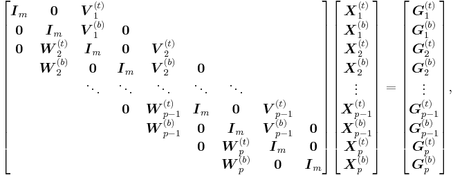
Notice that the system produced by the preprocessing stage can be reduced to a block pentadiagonal system of much smaller size (recall that  is much less than
  )
)
which we call the reduced system and denote by S̃X̃ = G̃.
Once all X (t)
j and X (b)
j are found, all X′j can be recovered with perfect parallelism via
SPIKE as a polyalgorithmic banded linear system solver
Despite being logically divided into two stages, computationally, the SPIKE algorithm comprises three stages:
- factorizing the diagonal blocks,
- computing the spikes,
- solving the reduced system.
Each of these stages can be accomplished in several ways, allowing a multitude of variants. Two notable variants are the recursive SPIKE algorithm for non-diagonally-dominant cases and the truncated SPIKE algorithm for diagonally-dominant cases. Depending on the variant, a system can be solved either exactly or approximately. In the latter case, SPIKE is used as a preconditioner for iterative schemes like Krylov subspace methods and iterative refinement.
Recursive SPIKE
Preprocessing stage
The first step of the preprocessing stage is to factorize the diagonal blocks Aj. For numerical stability, one can use LAPACK's XGBTRF routines to LU factorize them with partial pivoting. Alternatively, one can also factorize them without partial pivoting but with a "diagonal boosting" strategy. The latter method tackles the issue of singular diagonal blocks.
In concrete terms, the diagonal boosting strategy is as follows. Let 0ε denote a configurable "machine zero". In each step of LU factorization, we require that the pivot satisfy the condition
- |pivot| > 0ε‖A‖1.
If the pivot does not satisfy the condition, it is then boosted by
where ε is a positive parameter depending on the machine's unit roundoff, and the factorization continues with the boosted pivot. This can be achieved by modified versions of ScaLAPACK's XDBTRF routines. After the diagonal blocks are factorized, the spikes are computed and passed on to the postprocessing stage.
Postprocessing stage
The two-partition case
In the two-partition case, i.e., when p = 2, the reduced system S̃X̃ = G̃ has the form
An even smaller system can be extracted from the center:
which can be solved using the block LU factorization
Once X (b)
1 and X (t)
2 are found, X (t)
1 and X (b)
2 can be computed via
- X (t)
1 = G (t)
1 − V (t)
1 X (t)
2 , - X (b)
2 = G (b)
2 − W (b)
2 X (b)
1 .
The multiple-partition case
Assume that p is a power of two, i.e., p = 2d. Consider a block diagonal matrix
- D̃1 = diag(D̃ [1]
1 ,…,D̃ [1]
p/2 )
where
for k = 1,…,p/2. Notice that D̃1 essentially consists of diagonal blocks of order 4m extracted from S̃. Now we factorize S̃ as
- S̃ = D̃1S̃2.
The new matrix S̃2 has the form
Its structure is very similar to that of S̃2, only differing in the number of spikes and their height (their width stays the same at m). Thus, a similar factorization step can be performed on S̃2 to produce
- S̃2 = D̃2S̃3
and
- S̃ = D̃1D̃2S̃3.
Such factorization steps can be performed recursively. After d − 1 steps, we obtain the factorization
- S̃ = D̃1⋯D̃d−1S̃d,
where S̃d has only two spikes. The reduced system will then be solved via
- X̃ = S̃ −1
d D̃ −1
d−1 ⋯D̃ −1
1 G̃.
The block LU factorization technique in the two-partition case can be used to handle the solving steps involving D̃1, …, D̃d−1 and S̃d for they essentially solve multiple independent systems of generalized two-partition forms.
Generalization to cases where p is not a power of two is almost trivial.
Truncated SPIKE
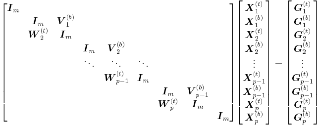
When A is diagonally-dominant, in the reduced system
the blocks V (t)
j and W (b)
j are often negligible. With them omitted, the reduced system becomes block diagonal
and can be easily solved in parallel.
The truncated SPIKE algorithm can be wrapped inside some outer iterative scheme (e.g., BiCGSTAB or iterative refinement) to improve the accuracy of the solution.
SPIKE as a preconditioner
The SPIKE algorithm can also function as a preconditioner for iterative methods for solving linear systems. To solve a linear system Ax = b using a SPIKE-preconditioned iterative solver, one extracts center bands from A to form a banded preconditioner M and solves linear systems involving M in each iteration with the SPIKE algorithm.
In order for the preconditioner to be effective, row and/or column permutation is usually necessary to move “heavy” elements of A close to the diagonal so that they are covered by the preconditioner. This can be accomplished by computing the weighted spectral reordering of A.
The SPIKE algorithm can be generalized by not restricting the preconditioner to be strictly banded. In particular, the diagonal block in each partition can be a general matrix and thus handled by a direct general linear system solver rather than a banded solver. This enhances the preconditioner, and hence allows better chance of convergence and reduces the number of iterations.
Implementations
Intel offers an implementation of the SPIKE algorithm under the name Intel Adaptive Spike-Based Solver.[1]
References
- Polizzi, E.; Sameh, A. H. (2006). "A parallel hybrid banded system solver: the SPIKE algorithm". Parallel Computing 32 (2): 177–194. doi:10.1016/j.parco.2005.07.005.
- Polizzi, E.; Sameh, A. H. (2007). "SPIKE: A parallel environment for solving banded linear systems". Computers & Fluids 36: 113–141. doi:10.1016/j.compfluid.2005.07.005.
- Mikkelsen, C. C. K.; Manguoglu, M (2008). "Analysis of the Truncated SPIKE Algorithm". SIAM Journal on Matrix Analysis and Applications 30 (4): 1500–1519. doi:10.1137/080719571.
- Manguoglu, M.; Sameh, A. H.; Schenk, O. (2009). "PSPIKE: A parallel hybrid sparse linear system solver". Euro-Par 2009 Parallel Processing. Lecture Notes in Computer Science 5704: 797–808. Bibcode 2009LNCS.5704..797M. doi:10.1007/978-3-642-03869-3_74. ISBN 978-3-642-03868-6.
- ^ "Intel Adaptive Spike-Based Solver - Intel Software Network". http://software.intel.com/en-us/articles/intel-adaptive-spike-based-solver/. Retrieved 2009-03-23.
- Sameh, A. H.; Kuck, D. J. (1978). "On Stable Parallel Linear System Solvers". Journal of the ACM 25: 81. doi:10.1145/322047.322054.
|
||||||||||||||


![\boldsymbol{\tilde{D}}_k^{[1]}=
\begin{bmatrix}
\boldsymbol{I}_m & \boldsymbol{0} & \boldsymbol{V}_{2k-1}^{(t)}\\
\boldsymbol{0} & \boldsymbol{I}_m & \boldsymbol{V}_{2k-1}^{(b)} & \boldsymbol{0}\\
\boldsymbol{0} & \boldsymbol{W}_{2k}^{(t)} & \boldsymbol{I}_m & \boldsymbol{0}\\
& \boldsymbol{W}_{2k}^{(b)} & \boldsymbol{0} & \boldsymbol{I}_m
\end{bmatrix}](/2012-wikipedia_en_all_nopic_01_2012/I/52a4690eaff402d59f9217d57779206c.png)
}\\
\boldsymbol{0} & \boldsymbol{I}_m & \boldsymbol{V}_1^{[2](b)} & \boldsymbol{0}\\
\boldsymbol{0} & \boldsymbol{W}_2^{[2](t)} & \boldsymbol{I}_m & \boldsymbol{0} & \boldsymbol{V}_2^{[2](t)}\\
& \boldsymbol{W}_2^{[2](b)} & \boldsymbol{0} & \boldsymbol{I}_{3m} & \boldsymbol{V}_2^{[2](b)} & \boldsymbol{0} \\
& & \ddots & \ddots & \ddots & \ddots & \ddots\\
& & & \boldsymbol{0} & \boldsymbol{W}_{p/2-1}^{[2](t)} & \boldsymbol{I}_{3m} & \boldsymbol{0} & \boldsymbol{V}_{p/2-1}^{[2](t)}\\
& & & & \boldsymbol{W}_{p/2-1}^{[2](b)} & \boldsymbol{0} & \boldsymbol{I}_m & \boldsymbol{V}_{p/2-1}^{[2](b)} & \boldsymbol{0}\\
& & & & & \boldsymbol{0} & \boldsymbol{W}_{p/2}^{[2](t)} & \boldsymbol{I}_m & \boldsymbol{0}\\
& & & & & & \boldsymbol{W}_{p/2}^{[2](b)} & \boldsymbol{0} & \boldsymbol{I}_{3m}
\end{bmatrix}\text{.}](/2012-wikipedia_en_all_nopic_01_2012/I/0402b5523f223aec17c2cc9dc2318079.png)
