Routh–Hurwitz stability criterion

The Routh–Hurwitz stability criterion is a necessary and sufficient method to establish the stability of a single-input, single-output (SISO), linear time invariant (LTI) control system. More generally, given a polynomial, some calculations using only the coefficients of that polynomial can lead to the conclusion that it is not stable. For the discrete case, see the Jury test equivalent.

The criterion establishes a systematic way to show that the linearized equations of motion of a system have only stable solutions exp(pt), that is where all p have negative real parts. It can be performed using either polynomial divisions or determinant calculus.

The criterion is derived through the use of the Euclidean algorithm and Sturm's theorem in evaluating Cauchy indices.

1 Using Euclid's algorithm
2 Using matrices
3 See also
4 References
5 External links

Using Euclid's algorithm

The criterion is related to Routh–Hurwitz theorem. Indeed, from the statement of that theorem, we have $p-q=w(%2B\infty)-w(-\infty)$ where:

p is the number of roots of the polynomial ƒ(z) with negative Real Part;
q is the number of roots of the polynomial ƒ(z) with positive Real Part (let us remind ourselves that ƒ is supposed to have no roots lying on the imaginary line);
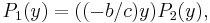
w(x) is the number of variations of the generalized Sturm chain obtained from $P_0(y)$ and $P_1(y)$ (by successive Euclidean divisions) where $f(iy)=P_0(y)%2BiP_1(y)$ for a real y.

By the fundamental theorem of algebra, each polynomial of degree n must have n roots in the complex plane (i.e., for an ƒ with no roots on the imaginary line, p + q = n). Thus, we have the condition that ƒ is a (Hurwitz) stable polynomial if and only if p − q = n (the proof is given below). Using the Routh–Hurwitz theorem, we can replace the condition on p and q by a condition on the generalized Sturm chain, which will give in turn a condition on the coefficients of ƒ.

Using matrices

Let f(z) be a complex polynomial. The process is as follows:

Compute the polynomials $P_0(y)$ and $P_1(y)$ such that $f(iy)=P_0(y)%2BiP_1(y)$ where y is a real number.
Compute the Sylvester matrix associated to $P_0(y)$ and $P_1(y)$ .
Rearrange each row in such a way that an odd row and the following one have the same number of leading zeros.
Compute each principal minor of that matrix.
If at least one of the minors is negative (or zero), then the polynomial f is not stable.

Example

Let $f(z)=az^2%2Bbz%2Bc$ (for the sake of simplicity we take real coefficients) where $c\neq 0$ (to avoid a root in zero so that we can use the Routh–Hurwitz theorem). First, we have to calculate the real polynomials $P_0(y)$ and $P_1(y)$ :

$f(iy)=-ay^2%2Biby%2Bc=P_0(y)%2BiP_1(y)=-ay^2%2Bc%2Bi(by).$

Next, we divide those polynomials to obtain the generalized Sturm chain:

- $P_0(y)=((-a/b)y)P_1(y)%2Bc,$ yields $P_2(y)=-c,$
- $P_1(y)=((-b/c)y)P_2(y),$ yields $P_3(y)=0$ and the Euclidean division stops.

Notice that we had to suppose b different from zero in the first division. The generalized Sturm chain is in this case $(P_0(y),P_1(y),P_2(y))=(c-ay^2,by,-c)$ . Putting $y=%2B\infty$ , the sign of $c-ay^2$ is the opposite sign of a and the sign of by is the sign of b. When we put $y=-\infty$ , the sign of the first element of the chain is again the opposite sign of a and the sign of by is the opposite sign of b. Finally, -c has always the opposite sign of c.

Suppose now that f is Hurwitz-stable. This means that $w(%2B\infty)-w(-\infty)=2$ (the degree of f). By the properties of the function w, this is the same as $w(%2B\infty)=2$ and $w(-\infty)=0$ . Thus, a, b and c must have the same sign. We have thus found the necessary condition of stability for polynomials of degree 2.

Routh–Hurwitz criterion for second, third, and fourth-order polynomials

For a second-order polynomial, 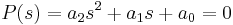$P(s) = a_2s^2 %2B a_1s %2B a_0 = 0$ , all the roots are in the left half plane (and the system with characteristic equation $P(s)$ is stable) if all the coefficients satisfy $a_n > 0$ .
For a third-order polynomial $P(s) = a_3s^3 %2B a_2s^2 %2B a_1s %2B a_0 = 0$ , all the coefficients must satisfy $a_n > 0$ , and $a_2a_1 > a_3a_0$
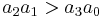
For a fourth-order polynomial $P(s) = a_4s^4 %2B a_3s^3 %2B a_2s^2 %2B a_1s %2B a_0 = 0$ , all the coefficients must satisfy $a_n 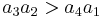> 0$ , and $a_3a_2 > a_4a_1$ and $a_3a_2a_1 > a_4a_1^2 %2B a_3^2a_0$

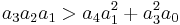
Higher-order example

A tabular method can be used to determine the stability when the roots of a higher order characteristic polynomial are difficult to obtain. For an nth-degree polynomial

$D(s)=a_ns^n%2Ba_{n-1}s^{n-1}%2B\cdots%2Ba_1s%2Ba_0$

the table has n + 1 rows and the following structure:

$a_n$	$a_{n-2}$	$a_{n-4}$	$\dots$
$a_{n-1}$	$a_{n-3}$	$a_{n-5}$	$\dots$
$b_1$	$b_2$	$b_3$	$\dots$
$c_1$	$c_2$	$c_3$	$\dots$
$\vdots$	$\vdots$	$\vdots$	$\ddots$

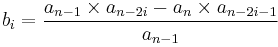
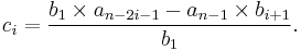
where the elements $b_i$ and $c_i$ can be computed as follows:

$b_i=\frac{a_{n-1}\times{a_{n-2i}}-a_n\times{a_{n-2i-1}}}{a_{n-1}}$
$c_i=\frac{b_1\times{a_{n-2i-1}}-a_{n-1}\times{b_{i%2B1}}}{b_1}.$

When completed, the number of sign changes in the first column will be the number of non-negative poles.

Consider a system with a characteristic polynomial

$D(s)=s^5%2B4s^4%2B2s^3%2B5s^2%2B3s%2B6.\,$

We have the following table:

1	2	3	0
4	5	6	0
0.75	1.5	0	0
−3	6	0
3	0
6	0

In the first column, there are two sign changes (0.75 → −3, and −3 → 3), thus there are two non-negative roots where the system is unstable. " Sometimes the presence of poles on the imaginary axis creates a situation of marginal stability. In that case the coefficients of the "Routh Array" become zero and thus further solution of the polynomial for finding changes in sign is not possible. Then another approach comes into play. The row of polynomial which is just above the row containing the zeroes is called "Auxiliary Polynomial".

$s^6%2B2s^5%2B8s^4%2B12s^3%2B20s^2%2B16s%2B16=0.\,$

We have the following table:

1	8	20	16
2	12	16	0
2	12	16	0
0	0	0	0

In such a case the Auxiliary polynomial is 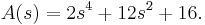$A(s)=2s^4%2B12s^2%2B16.\,$ which is again equal to zero. The next step is to differentiate the above equation which yields the following polynomial. 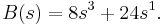$B(s)=8s^3%2B24s^1.\,$ . The coefficients of the row containing zero now become "8" and "24". The process of Routh array is proceeded using these values which yield two points on the imaginary axis. These two points on the imaginary axis are the prime cause of marginal stability.^[1]

References

^ Saeed, Syed Hasan (2008). Automatic Control Systems. Delhi: Katson Publishers. pp. 206, 207. ISBN 978-81-906919-2-5.

Hurwitz, A. (1964). "‘On the conditions under which an equation has only roots with negative real parts". Selected Papers on Mathematical Trends in Control Theory.

Routh, E. J. (1877). A Treatise on the Stability of a Given State of Motion: Particularly Steady Motion. Macmillan and co..

Gantmacher, F. R. (1959). "Applications of the Theory of Matrices". Interscience, New York 641 (9): 1–8.

Pippard, A. B.; Dicke, R. H. (1986). "Response and Stability, An Introduction to the Physical Theory". American Journal of Physics 54: 1052. doi:10.1119/1.14826. http://link.aip.org/link/?AJPIAS/54/1052/1. Retrieved 2008-05-07.
Weisstein, Eric W. "Routh-Hurwitz Theorem.". MathWorld--A Wolfram Web Resource. http://mathworld.wolfram.com/Routh-HurwitzTheorem.html.

Richard C. Dorf, Robert H. Bishop (2001). Modern Control Systems, 9th Edition. Prentice Hall. ISBN 0-13-030660-6.

External links

A MATLAB script implementing the Routh-Hurwitz test