Low-discrepancy sequence

In mathematics, a low-discrepancy sequence is a sequence with the property that for all values of N, its subsequence x₁, ..., x_N has a low discrepancy.

Roughly speaking, the discrepancy of a sequence is low if the number of points in the sequence falling into an arbitrary set B is close to proportional to the measure of B, as would happen on average (but not for particular samples) in the case of a uniform distribution. Specific definitions of discrepancy differ regarding the choice of B (hyperspheres, hypercubes, etc.) and how the discrepancy for every B is computed (usually normalized) and combined (usually by taking the worst value).

Low-discrepancy sequences are also called quasi-random or sub-random sequences, due to their common use as a replacement of uniformly distributed random numbers. The "quasi" modifier is used to denote more clearly that the values of a low-discrepancy sequence are neither random nor pseudorandom, but such sequences share some properties of random variables and in certain applications such as the quasi-Monte Carlo method their lower discrepancy is an important advantage.

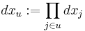
At least three methods of numerical integration can be phrased as follows. Given a set {x₁, ..., x_N} in the interval [0,1], approximate the integral of a function f as the average of the function evaluated at those points:

$\int_0^1 f(u)\,du \approx \frac{1}{N}\,\sum_{i=1}^N f(x_i).$

If the points are chosen as x_i = i/N, this is the rectangle rule. If the points are chosen to be randomly (or pseudorandomly) distributed, this is the Monte Carlo method. If the points are chosen as elements of a low-discrepancy sequence, this is the quasi-Monte Carlo method. A remarkable result, the Koksma–Hlawka inequality (stated below), shows that the error of such a method can be bounded by the product of two terms, one of which depends only on f, and the other one is the discrepancy of the set {x₁, ..., x_N}.

It is convenient to construct the set {x₁, ..., x_N} in such a way that if a set with N+1 elements is constructed, the previous N elements need not be recomputed. The rectangle rule uses points set which have low discrepancy, but in general the elements must be recomputed if N is increased. Elements need not be recomputed in the Monte Carlo method if N is increased, but the point sets do not have minimal discrepancy. By using low-discrepancy sequences, the quasi-Monte Carlo method has the desirable features of the other two methods.

1 Definition of discrepancy
2 Graphical examples
3 The Koksma–Hlawka inequality
4 The formula of Hlawka-Zaremba
5 The version of the Koksma–Hlawka inequality
6 The Erdős–Turan–Koksma inequality
7 The main conjectures
8 The best-known sequences
9 Lower bounds
10 Applications
11 References
12 External links

Definition of discrepancy

The discrepancy of a set P = {x₁, ..., x_N} is defined, using Niederreiter's notation, as

$D_N(P) = \sup_{B\in J} \left| \frac{A(B;P)}{N} - \lambda_s(B) \right|$

where λ_s is the s-dimensional Lebesgue measure, A(B;P) is the number of points in P that fall into B, and J is the set of s-dimensional intervals or boxes of the form

$\prod_{i=1}^s [a_i, b_i) = \{ \mathbf{x} \in \mathbf{R}^s�: a_i \le x_i < b_i \} \,$

where $0 \le a_i < b_i \le 1$ .

The star-discrepancy D^*_N(P) is defined similarly, except that the supremum is taken over the set J^* of intervals of the form

$\prod_{i=1}^s [0, u_i)$

where u_i is in the half-open interval [0, 1).

The two are related by

$D^*_N \le D_N \le 2^s D^*_N . \,$

Graphical examples

The points plotted below are the first 100, 1000, and 10000 elements in a sequence of the Sobol' type. For comparison, 10000 elements of a sequence of pseudorandom points are also shown. The low-discrepancy sequence was generated by TOMS algorithm 659^[1]. An implementation of the algorithm in Fortran is available from Netlib.

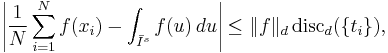
The Koksma–Hlawka inequality

Let Ī^s be the s-dimensional unit cube, Ī^s = [0, 1] × ... × [0, 1]. Let f have bounded variation V(f) on Ī^s in the sense of Hardy and Krause. Then for any x₁, ..., x_N in I^s = [0, 1) × ... × [0, 1),

$\left| \frac{1}{N} \sum_{i=1}^N f(x_i) - \int_{\bar I^s} f(u)\,du \right| \le V(f)\, D_N^* (x_1,\ldots,x_N).$

The Koksma-Hlawka inequality is sharp in the following sense: For any point set {x₁,...,x_N} in I^s and any $\epsilon>0$ , there is a function f with bounded variation and V(f)=1 such that

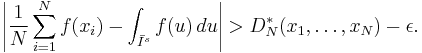
$\left| \frac{1}{N} \sum_{i=1}^N f(x_i) - \int_{\bar I^s} f(u)\,du \right|>D_{N}^{*}(x_1,\ldots,x_N)-\epsilon.$

Therefore, the quality of a numerical integration rule depends only on the discrepancy D^*_N(x₁,...,x_N).

The formula of Hlawka-Zaremba

Let $D=\{1,2,\ldots,d\}$ . For $\emptyset\neq u\subseteq D$ we write

$dx_u:=\prod_{j\in u} dx_j$

and denote by $(x_u,1)$ the point obtained from x by replacing the coordinates not in u by $1$ . Then

$\frac{1}{N} \sum_{i=1}^N f(x_i) - \int_{\bar I^s} f(u)\,du= \sum_{\emptyset\neq u\subseteq D}(-1)^{|u|} \int_{[0,1]^{|u|}}{\rm disc}(x_u,1)\frac{\partial^{|u|}}{\partial x_u}f(x_u,1) dx_u.$

The $L^2$ version of the Koksma–Hlawka inequality

Applying the Cauchy-Schwarz inequality for integrals and sums to the Hlawka-Zaremba identity, we obtain an $L^2$ version of the Koksma–Hlawka inequality:

$\left|\frac{1}{N} \sum_{i=1}^N f(x_i) - \int_{\bar I^s} f(u)\,du\right|\le \|f\|_{d}\,{\rm disc}_{d}(\{t_i\}),$

where

${\rm disc}_{d}(\{t_i\})=\left(\sum_{\emptyset\neq u\subseteq D} \int_{[0,1]^{|u|}}{\rm disc}(x_u,1)^2 dx_u\right)^{1/2}$

and

$\|f\|_{d}=\left(\sum_{u\subseteq D} \int_{[0,1]^{|u|}} \left|\frac{\partial^{|u|}}{\partial x_u}f(x_u,1)\right|^2 dx_u\right)^{1/2}.$

The Erdős–Turan–Koksma inequality

It is computationally hard to find the exact value of the discrepancy of large point sets. The Erdős–Turán–Koksma inequality provides an upper bound.

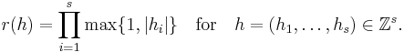
Let x₁,...,x_N be points in I^s and H be an arbitrary positive integer. Then

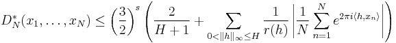
$D_{N}^{*}(x_1,\ldots,x_N)\leq \left(\frac{3}{2}\right)^s \left( \frac{2}{H%2B1}%2B \sum_{0<\|h\|_{\infty}\leq H}\frac{1}{r(h)} \left| \frac{1}{N} \sum_{n=1}^{N} e^{2\pi i\langle h,x_n\rangle} \right| \right)$

where

$r(h)=\prod_{i=1}^s\max\{1,|h_i|\}\quad\mbox{for}\quad h=(h_1,\ldots,h_s)\in\Z^s.$

The main conjectures

Conjecture 1. There is a constant c_s depending only on the dimension s, such that

$D_{N}^{*}(x_1,\ldots,x_N)\geq c_s\frac{(\ln N)^{s-1}}{N}$

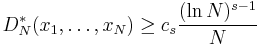
for any finite point set {x₁,...,x_N}.

Conjecture 2. There is a constant c^'_s depending only on s, such that

$D_{N}^{*}(x_1,\ldots,x_N)\geq c'_s\frac{(\ln N)^{s}}{N}$

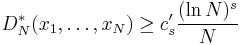
for any infinite sequence x₁,x₂,x₃,....

These conjectures are equivalent. They have been proved for s ≤ 2 by W. M. Schmidt. In higher dimensions, the corresponding problem is still open. The best-known lower bounds are due to K. F. Roth.

The best-known sequences

Constructions of sequences are known such that

$D_{N}^{*}(x_1,\ldots,x_N)\leq C\frac{(\ln N)^{s}}{N}.$

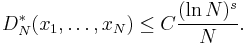
where C is a certain constant, depending on the sequence. After Conjecture 2, these sequences are believed to have the best possible order of convergence. See also: van der Corput sequence, Halton sequences, Sobol sequences.

Lower bounds

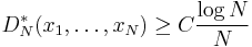
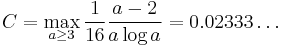
Let s = 1. Then

$D_N^*(x_1,\ldots,x_N)\geq\frac{1}{2N}$

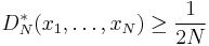
for any finite point set {x₁, ..., x_N}.

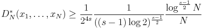
Let s = 2. W. M. Schmidt proved that for any finite point set {x₁, ..., x_N},

$D_N^*(x_1,\ldots,x_N)\geq C\frac{\log N}{N}$

where

$C=\max_{a\geq3}\frac{1}{16}\frac{a-2}{a\log a}=0.02333\dots$

For arbitrary dimensions s > 1, K.F. Roth proved that

$D_N^*(x_1,\ldots,x_N)\geq\frac{1}{2^{4s}}\frac{1}{((s-1)\log2)^\frac{s-1}{2}}\frac{\log^{\frac{s-1}{2}}N}{N}$

for any finite point set {x₁, ..., x_N}. This bound is the best known for s > 3.

Applications

References

Kuipers, L.; Niederreiter, H. (2005), Uniform distribution of sequences, Dover Publications, ISBN 0-486-45019-8
Harald Niederreiter. Random Number Generation and Quasi-Monte Carlo Methods. Society for Industrial and Applied Mathematics, 1992. ISBN 0-89871-295-5
Michael Drmota and Robert F. Tichy, Sequences, discrepancies and applications, Lecture Notes in Math., 1651, Springer, Berlin, 1997, ISBN 3-540-62606-9
William H. Press, Brian P. Flannery, Saul A. Teukolsky, William T. Vetterling. Numerical Recipes in C. Cambridge, UK: Cambridge University Press, second edition 1992. ISBN 0-521-43108-5 (see Section 7.7 for a less technical discussion of low-discrepancy sequences)
Quasi-Monte Carlo Simulations, http://www.puc-rio.br/marco.ind/quasi_mc.html

External links

Collected Algorithms of the ACM (See algorithms 647, 659, and 738.)
GNU Scientific Library Quasi-Random Sequences

^ P. Bratley and B.L. Fox in ACM Transactions on Mathematical Software, vol. 14, no. 1, pp 88—100

Low-discrepancy sequence

Contents

Definition of discrepancy

Graphical examples

The Koksma–Hlawka inequality

The formula of Hlawka-Zaremba

The version of the Koksma–Hlawka inequality

The Erdős–Turan–Koksma inequality

The main conjectures

The best-known sequences

Lower bounds

Applications

References

External links

The $L^2$ version of the Koksma–Hlawka inequality