Quantile

Quantiles are points taken at regular intervals from the cumulative distribution function (CDF) of a random variable. Dividing ordered data into $q$ essentially equal-sized data subsets is the motivation for $q$ -quantiles; the quantiles are the data values marking the boundaries between consecutive subsets. Put another way, the $k^\mathrm{th}$ $q$ -quantile for a random variable is the value $x$ such that the probability that the random variable will be less than $x$ is at most $k/q$ and the probability that the random variable will be more than $x$ is at most $(q-k)/q$ . There are $q-1$ of the $q$ -quantiles, one for each integer $k$ satisfying $0 < k < q$ .

1 Specialized quantiles
2 Quantiles of a population
3 Examples
- 3.1 Even-sized population
- 3.2 Odd-sized population
4 Discussion
5 Estimating the quantiles of a population
6 See also
7 References

Specialized quantiles

Some q-quantiles have special names:

The 2-quantile is called the median
The 3-quantiles are called tertiles or terciles → T
The 4-quantiles are called quartiles → Q
The 5-quantiles are called quintiles → QU
The 6-quantiles are called sextiles → S
The 10-quantiles are called deciles → D
The 12-quantiles are called duo-deciles → Dd
The 20-quantiles are called vigintiles → V
The 100-quantiles are called percentiles → P
The 1000-quantiles are called permilles → Pr

More generally, one can consider the quantile function for any distribution. This is defined for real variables between zero and one and is mathematically the inverse of the cumulative distribution function.

Quantiles of a population

For a population of discrete values or for a continuous population density, the $k$ th $q$ -quantile is the data value where the cumulative distribution function crosses $k/q$ . That $x$ is a $k$ th $q$ -quantile for a variable $X$ if

$\Pr[X < x] \le k/q$ (or, equivalently, $\Pr[X \ge x] \ge 1-k/q$ )

and

$\Pr[X \le x] \ge k/q$ (or, equivalently, $\Pr[X > x] \le 1-k/q$ ).

For a finite population of $N$ values indexed 1,..., $N$ from lowest to highest, the $k$ th $q$ -quantile of this population can be computed via the value of $I_p = N \frac{k}{q}$ . If $I_p$ is not an integer, then round up to the next integer to get the appropriate index; the corresponding data value is the $k$ th $q$ -quantile. On the other hand, if $I_p$ is an integer then any number from the data value at that index to the data value of the next can be taken as the quantile, and it is conventional (though arbitrary) to take the average of those two values (see Estimating the quantiles).

If, instead of using integers $k$ and $q$ , the “ $p$ -quantile” is based on a real number $p$ with $0<p<1$ , then $p$ replaces $k/q$ in the above formulae. Some software programs (including Microsoft Excel) regard the minimum and maximum as the 0th and 100th percentile, respectively; however, such terminology is an extension beyond traditional statistics definitions.

Examples

Even-sized population

Consider an ordered population of 10 data values {3, 6, 7, 8, 8, 10, 13, 15, 16, 20}.

The rank of the first quartile is 10×(1/4) = 2.5, which rounds up to 3, meaning that 3 is the rank in the population (from least to greatest values) at which approximately 1/4 of the values are less than the value of the first quartile. The third value in the population is 7.
The rank of the second quartile (same as the median) is 10×(2/4) = 5, which is an integer, while the number of values (10) is an even number, so the average of both the fifth and sixth values is taken—that is (8+10)/2 = 9, though any value from 8 through to 10 could be taken to be the median.
The rank of the third quartile is 10×(3/4) = 7.5, which rounds up to 8. The eighth value in the population is 15.

Odd-sized population

Consider an ordered population of 11 data values {3, 6, 7, 8, 8, 9, 10, 13, 15, 16, 20}.

The first quartile is determined by 11×(1/4) = 2.75, which rounds up to 3, meaning that 3 is the rank in the population (from least to greatest values) at which approximately 1/4 of the values are less than the value of the first quartile. The third value in the population is 7.
The second quartile value (same as the median) is determined by 11×(2/4) = 5.5, which rounds up to 6. Therefore 6 is the rank in the population (from least to greatest values) at which approximately 2/4 of the values are less than the value of the second quartile (or median). The sixth value in the population is 9.
The third quartile value for the original example above is determined by 11×(3/4) = 8.25, which rounds up to 9. The ninth value in the population is 15.

Discussion

Standardized test results are commonly misinterpreted as a student scoring "in the 80th percentile," for example, as if the 80th percentile is an interval to score "in," which it is not; one can score "at" some percentile, or between two percentiles, but not "in" some percentile. Perhaps by this example it is meant that the student scores between the 80th and 81st percentiles.

If a distribution is symmetric, then the median is the mean (so long as the latter exists). But, in general, the median and the mean differ. For instance, with a random variable that has an exponential distribution, any particular sample of this random variable will have roughly a 63% chance of being less than the mean. This is because the exponential distribution has a long tail for positive values but is zero for negative numbers.

Quantiles are useful measures because they are less susceptible to long-tailed distributions and outliers. Empirically, if the data being analyzed are not actually distributed according to an assumed distribution, or if there are other potential sources for outliers that are far removed from the mean, then quantiles may be more useful descriptive statistics than means and other moment-related statistics.

Closely related is the subject of least absolute deviations, a method of regression that is more robust to outliers than is least squares, in which the sum of the absolute value of the observed errors is used in place of the squared error. The connection is that the mean is the single estimate of a distribution that minimizes expected squared error while the median minimizes expected absolute error. Least absolute deviations shares the ability to be relatively insensitive to large deviations in outlying observations, although even better methods of robust regression are available.

The quantiles of a random variable are preserved under increasing transformations, in the sense that, for example, if $m$ is the median of a random variable $X$ , then $2^m$ is the median of $2^X$ , unless an arbitrary choice has been made from a range of values to specify a particular quantile. (See quantile estimation, below, for examples of such interpolation.) Quantiles can also be used in cases where only ordinal data are available.

Estimating the quantiles of a population

There are several methods for estimating the quantiles.^[1] The most comprehensive breadth of methods is available in the R programming language, which includes nine sample quantile methods.^[2] SAS includes five sample quantile methods, STATA includes two, and Microsoft Excel includes one.

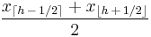
In effect, the methods compute Q_p, the estimate for the kth q-quantile, where p = k / q, from a sample of size N by computing a real valued index h. When h is an integer, the hth smallest of the N values, x_h, is the quantile estimate. Otherwise a rounding or interpolation scheme is used to compute the quantile estimate from h, x_⌊h⌋, and x_⌈h⌉. (For notation, see floor and ceiling functions).

Estimate types include:

Type	h	Q_p	Notes
R-1, SAS-3	$Np %2B 1/2\,$	$x_{\lceil h\,-\,1/2 \rceil}$	Inverse of empirical distribution function. When p = 0, use x₁.
R-2, SAS-5	$Np %2B 1/2\,$	$\frac{x_{\lceil h\,-\,1/2 \rceil} %2B x_{\lfloor h\,%2B\,1/2 \rfloor}}{2}$	The same as R-1, but with averaging at discontinuities. When p = 0, x₁. When p = 1, use x_N.
R-3, SAS-2	$Np\,$	$x_{\lfloor h \rceil}\,$	The observation numbered closest to Np. Here, ⌊ h ⌉ indicates rounding to the nearest integer, choosing the even integer in the case of a tie. When p ≤ (1/2) / N, use x₁.
R-4, SAS-1	$Np\,$	$x_{\lfloor h \rfloor} %2B (h - \lfloor h \rfloor) (x_{\lfloor h \rfloor %2B 1} - x_{\lfloor h \rfloor})$	Linear interpolation of the empirical distribution function. When p < 1 / N, use x₁. When p = 1, use x_N.
R-5	$Np %2B 1/2\,$	$x_{\lfloor h \rfloor} %2B (h - \lfloor h \rfloor) (x_{\lfloor h \rfloor %2B 1} - x_{\lfloor h \rfloor})$	Piecewise linear function where the knots are the values midway through the steps of the empirical distribution function. When p < (1/2) / N, use x₁. When p ≥ (N - 1/2) / N, use x_N.
R-6, SAS-4	$(N%2B1)p\,$	$x_{\lfloor h \rfloor} %2B (h - \lfloor h \rfloor) (x_{\lfloor h \rfloor %2B 1} - x_{\lfloor h \rfloor})$	Linear interpolation of the expectations for the order statistics for the uniform distribution on [0,1]. When p < 1 / (N+1), use x₁. When p ≥ N / (N + 1), use x_N.
R-7, Excel	$(N-1)p %2B 1\,$	$x_{\lfloor h \rfloor} %2B (h - \lfloor h \rfloor) (x_{\lfloor h \rfloor %2B 1} - x_{\lfloor h \rfloor})$	Linear interpolation of the modes for the order statistics for the uniform distribution on [0,1]. When p = 1, use x_N.
R-8	$(N %2B 1/3)p %2B 1/3\,$	$x_{\lfloor h \rfloor} %2B (h - \lfloor h \rfloor) (x_{\lfloor h \rfloor %2B 1} - x_{\lfloor h \rfloor})$	Linear interpolation of the approximate medians for order statistics. When p < (2/3) / (N + 1/3), use x₁. When p ≥ (N - 1/3) / (N + 1/3), use x_N.
R-9	$(N %2B 1/4)p %2B 3/8\,$	$x_{\lfloor h \rfloor} %2B (h - \lfloor h \rfloor) (x_{\lfloor h \rfloor %2B 1} - x_{\lfloor h \rfloor})$	The resulting quantile estimates are approximately unbiased for the expected order statistics if x is normally distributed. When p < (5/8) / (N + 1/4), use x₁. When p ≥ (N - 3/8) / (N + 1/4), use x_N.
	$(N %2B 2)p - 1/2\,$	$x_{\lfloor h \rfloor} %2B (h - \lfloor h \rfloor) (x_{\lfloor h \rfloor %2B 1} - x_{\lfloor h \rfloor})$	If h were rounded, this would give the order statistic with the least expected square deviation relative to p. When p < (3/2) / (N + 2), use x₁. When p ≥ (N + 1/2) / (N + 2), use x_N.

Note that R-3 and R-4 do not give h = (N + 1) / 2 when p = 1/2.

The standard error of a quantile estimate can in general be estimated via the bootstrap. The Maritz-Jarrett method can also be used.^[3] Note that a Bayesian approach to quantile estimation (along with a credible interval) fails with an improper prior and a proper prior is required.

References

R.J. Serfling. Approximation Theorems of Mathematical Statistics. John Wiley & Sons, 1980.

^ Hyndman, R.J.; Fan, Y. (November 1996). "Sample Quantiles in Statistical Packages". American Statistician (American Statistical Association) 50 (4): 361–365. doi:10.2307/2684934. JSTOR 2684934.
^ Frohne, I.; Hyndman, R.J. (2009). Sample Quantiles. R Project. ISBN 3-900051-07-0. http://stat.ethz.ch/R-manual/R-devel/library/stats/html/quantile.html.
^ Rand R. Wilcox. Introduction to robust estimation and hypothesis testing. ISBN 0127515429