Preference Ranking Organization Method for Enrichment Evaluation
The Preference Ranking Organization Method for Enrichment of Evaluations and its descriptive complement Geometrical Analysis for Interactive Aid are better known as the PROMETHEE & GAIA[1] methods. They are multi-criteria decision aid methods that belong to the family of the outranking methods initiated by Professor Bernard Roy with the ELECTRE methods. An original aspect of the PROMETHEE and GAIA methods is that they offer complementary descriptive and prescriptive approaches to the analysis of discrete multicriteria problems including a number of actions (decisions) evaluated on several criteria.
The descriptive approach, named GAIA,[2] allows the decision maker to visualize the main features of a decision problem: he/she is able to easily identify conflicts or synergies between criteria, to identify clusters of actions and to highlight remarkable performances.
The prescriptive approach, named PROMETHEE,[3] provides the decision maker with both complete and partial rankings of the actions.
The basic elements of the PROMETHEE method have been first introduced by Professor Jean-Pierre Brans (CSOO, VUB Vrije Universiteit Brussel) in 1982.[4] It was later developed and implemented by Professor Jean-Pierre Brans and Professor Bertrand Mareschal (Solvay Brussels School of Economics and Management, ULB Université Libre de Bruxelles), including extensions such as GAIA.
PROMETHEE has successfully been used in many decision making contexts worldwide. A non-exhaustive list of scientific publications about extensions, applications and discussions related to the PROMETHEE methods[5] has recently been published.
The PROMETHEE methods have been implemented in several interactive computer software such as PROMCALC, DECISION LAB 2000, D-Sight and PROMETHEE.
Contents |
The Model
Assumptions
Let  be a set of n actions and let
  be a consistent family of q criteria. Without loss of generality, we will assume that these criteria have to be maximized.
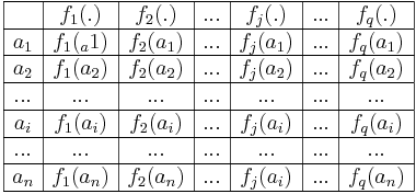
The basic data related to such a problem can be written in a table containing  evaluations. Each line corresponds to an action and each column corresponds to a criterion.
Pairwise Comparisons
At first, pairwise comparisons will be made between all the actions for each criterion:
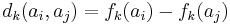
 is the difference between the evaluations of two actions for criterion
  . Of course, these differences depend on the measurement scales used and are not always easy to compare for the decision maker.
Preference Degree
As a consequence the notion of preference function is introduced to translate the difference into a unicriterion preference degree as follows:
![\pi_k(a_i,a_j)=P_k[d_k(a_i,a_j)]](/2012-wikipedia_en_all_nopic_01_2012/I/09ef66a01149b903e5a5d55fda95f518.png)
where ![P_k:\R\rightarrow[0,1]](/2012-wikipedia_en_all_nopic_01_2012/I/ea5ab9a298890e44093e3b763f87a73d.png) is a positive non-decreasing preference function such that
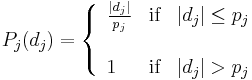
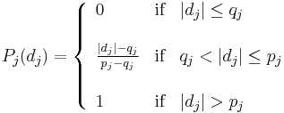
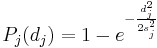
is a positive non-decreasing preference function such that  . Six different types of preference function are proposed in the original PROMETHEE definition. Among them, the linear unicriterion preference function is often used in practice for quantitative criteria:
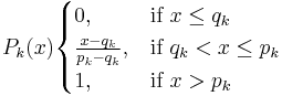
where  and
and  are respectively the indifference and preference thresholds. The meaning of these parameters is the following: when the difference is smaller than the indifference threshold it is considered as negligible by the decision maker. Therefore the corresponding unicriterion preference degree is equal to zero. If the difference exceeds the preference threshold it is considered to be significant. Therefore the unicriterion preference degree is equal to one (the maximum value). When the difference is between the two thresholds, an intermediate value is computed for the preference degree using a linear interpolation.
Multicriteria Preference Degree
When a preference function has been associated to each criterion by the decision maker, all comparisons between all pairs of actions can be done for all the criteria. A multicriteria preference degree is then computed to globally compare every couple of actions:
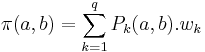
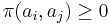
Where  represents the weight of criterion . It is assumed that
  and
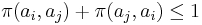
and  . As a direct consequence, we have:
Multicriteria Preference Flows
In order to position every action a with respect to all the other actions, two scores are computed:
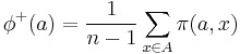
The positive preference flow  quantifies how a given action
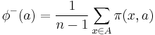
  is globally preferred to all the other actions while the negative preference flow
  quantifies how a given action is being globally preferred by all the other actions. An ideal action would have a positive preference flow equal to 1 and a negative preference flow equal to 0. The two preference flows induce two generally different complete rankings on the set of actions. The first one is obtained by ranking the actions according to the decreasing values of their positive flow scores. The second one is obtained by ranking the actions according to the increasing values of their negative flow scores. The Promethee I partial ranking is defined as the intersection of these two rankings. As a consequence, an action will be as good as another action
  if
if  and
and 
The positive and negative preference flows are aggregated into the net preference flow:
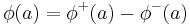
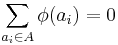
Direct consequences of the previous formula are:
![\phi(a_i) \in [-1;1]](/2012-wikipedia_en_all_nopic_01_2012/I/0030bb26a1c340135b60077523e7b043.png)
The Promethee II complete ranking is obtained by ordering the actions according to the decreasing values of the net flow scores.
Unicriterion net flows
According to the definition of the multicriteria preference degree, the multicriteria net flow can be disaggregated as follows:
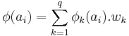
where:
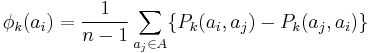 .
.
The unicriterion net flow, denoted ![\phi_{k}(a_i)\in[-1;1]](/2012-wikipedia_en_all_nopic_01_2012/I/3291d549c0f714f0758c6ef42dcc00e8.png) , has the same interpretation as the multicriteria net flow
, has the same interpretation as the multicriteria net flow  but is limited to one single criterion. Any action can be characterized by a vector
 ![\vec \phi(a_i) =[\phi_1(a_i),...,\phi_k(a_i),\phi_q(a_i)]](/2012-wikipedia_en_all_nopic_01_2012/I/c2b1bd1b82c24cb1f8b2699c120b9b32.png) in a
in a  dimensional space. The GAIA plane is the principal plane obtained by applying a principal components analysis to the set of actions in this space.
PROMETHEE Preference Functions
- Usual
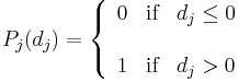
- U-Shape
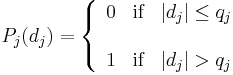
- V-Shape
- Level
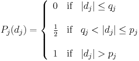
- Linear
- Gaussian
PROMETHEE Rankings
PROMETHEE I
PROMETHEE I is a partial ranking of the actions. It is based on the positive and negative flows. It includes preferences, indifferences and incomparabilities (partial preorder).
PROMETHEE II
PROMETHEE II is a complete ranking of the actions. It is based on the multicriteria net flow. It includes preferences and indifferences (preorder).
See also
- Decision making
- Decision making software
- D-Sight
- Multi-Criteria Decision Analysis
- Pairwise comparison
- Preference
References
- ^ J. Figueira, S. Greco, and M. Ehrgott (2005). Multiple Criteria Decision Analysis: State of the Art Surveys. Springer Verlag.
- ^ B. Mareschal, J.P. Brans (1988). "Geometrical representations for MCDA. the GAIA module". European Journal of Operational Research.
- ^ J.P. Brans and P. Vincke (1985). "A preference ranking organisation method: The PROMETHEE method for MCDM". Management Science.
- ^ J.P. Brans (1982). "L’ingénierie de la décision: élaboration d’instruments d’aide à la décision. La méthode PROMETHEE.". Presses de l’Université Laval.
- ^ M. Behzadian, R.B. Kazemzadeh, A. Albadvi and M. Aghdasi (2010). "PROMETHEE: A comprehensive literature review on methodologies and applications". European Journal of Operational Research.