Monotone cubic interpolation
In the mathematical subfield of numerical analysis, monotone cubic interpolation is a variant of cubic interpolation that preserves monotonicity of the data set being interpolated.
Monotonicity is preserved by linear interpolation but not guaranteed by cubic interpolation.
Contents |
Monotone cubic Hermite interpolation
Monotone interpolation can be accomplished using cubic Hermite spline with the tangents  modified to ensure the monotonicity of the resulting Hermite spline.
Interpolant selection
There are several ways of selecting interpolating tangents for each data point. This section will outline the use of the Fritsch–Carlson method.
Let the data points be  for
for 
- Compute the slopes of the secant lines between successive points:
for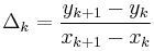
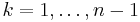 .
. - Initialize the tangents at every data point as the average of the secants,
for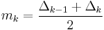
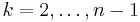 ; these may be updated in further steps. For the endpoints, use one-sided differences:

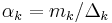
- For , if
 (if two successive
  are equal), then set
 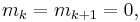 as the spline connecting these points must be flat to preserve monotonicity. Ignore step 4 and 5 for those
  .
. - Let
 and
and 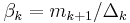 . If
. If  or
or  are computed to be less than zero, then the input data points are not strictly monotone. In such cases, piecewise monotone curves can still be generated by choosing
 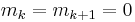 , although global strict monotonicity is not possible.
 - To prevent overshoot and ensure monotonicity, the function
must have a value greater than (or equal to, if monotonicity need not be strict) zero. One simple way to satisfy this constraint is to restrict the magnitude of vector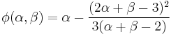
 to a circle of radius 3. That is, if
 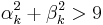 , then set
 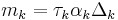 and
and 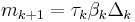 where
where 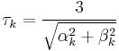 .
.
Note that only one pass of the algorithm is required.
Cubic interpolation
After the preprocessing, evaluation of the interpolated spline is equivalent to cubic Hermite spline, using the data  ,
,  , and
, and  for .
for .
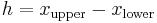
To evaluate at  , find the smallest value larger than ,
  , and the largest value smaller than ,
  , among such that
 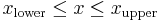 . Calculate
 and
and 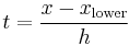
then the interpolant is

where  are the basis functions for the cubic Hermite spline.
External links
- GPLv3 licensed C++ implementation: MonotCubicInterpolator.cpp MonotCubicInterpolator.hpp
References
- Fritsch, F. N.; Carlson, R. E. (1980). "Monotone Piecewise Cubic Interpolation". SIAM Journal on Numerical Analysis (SIAM) 17 (2): 238–246. doi:10.1137/0717021.