Merge sort
An example on Merge sort. First divide the list into the smallest unit (1 element), then compare each element with the adjacent list to sort and merge the two adjacent list. Finally all the elements are sorted and merged. |
|
| Class | Sorting algorithm |
|---|---|
| Data structure | Array |
| Worst case performance | O(n log n) |
| Best case performance |
O(n log n) typical, O(n) natural variant |
| Average case performance | O(n log n) |
| Worst case space complexity | O(n) auxiliary |
Merge sort is an O(n log n) comparison-based sorting algorithm. Most implementations produce a stable sort, meaning that the implementation preserves the input order of equal elements in the sorted output. It is a divide and conquer algorithm. Merge sort was invented by John von Neumann in 1945.[1] A detailed description and analysis of bottom-up mergesort appeared in a report by Goldstine and Neumann as early as 1948.[2]
Contents |
Algorithm
Conceptually, a merge sort works as follows
- If the list is of length 0 or 1, then it is already sorted. Otherwise:
- Divide the unsorted list into two sublists of about half the size.
- Sort each sublist recursively by re-applying the merge sort.
- Merge the two sublists back into one sorted list.
Merge sort incorporates two main ideas to improve its runtime:
- A small list will take fewer steps to sort than a large list.
- Fewer steps are required to construct a sorted list from two sorted lists than from two unsorted lists. For example, you only have to traverse each list once if they're already sorted (see the merge function below for an example implementation).
Example: Use merge sort to sort a list of integers contained in an array:
Suppose we have an array A with n indices ranging from  to
to  . We apply merge sort to
  and
and  where c is the integer part of
  . When the two halves are returned they will have been sorted. They can now be merged to form a sorted array.
In a simple pseudocode form, the algorithm could look something like this:
function merge_sort(m)
    if length(m) ≤ 1
        return m
    var list left, right, result
    var integer middle = length(m) / 2
    for each x in m up to middle
         add x to left
    for each x in m after or equal middle
         add x to right
    left = merge_sort(left)
    right = merge_sort(right)
    result = merge(left, right)
    return result
The merge function needs to then merge both the left and right lists. It has several variations; one is shown:
function merge(left,right)
    var list result
    while length(left) > 0 or length(right) > 0
        if length(left) > 0 and length(right) > 0
            if first(left) ≤ first(right)
                append first(left) to result
                left = rest(left)
            else
                append first(right) to result
                right = rest(right)
        else if length(left) > 0
            append first(left) to result
            left = rest(left)
        else if length(right) > 0
            append first(right) to result
            right = rest(right)
    end while
    return result
Analysis
In sorting n objects, merge sort has an average and worst-case performance of O(n log n). If the running time of merge sort for a list of length n is T(n), then the recurrence T(n) = 2T(n/2) + n follows from the definition of the algorithm (apply the algorithm to two lists of half the size of the original list, and add the n steps taken to merge the resulting two lists). The closed form follows from the master theorem.
In the worst case, the number of comparisons merge sort makes is equal to or slightly smaller than (n ⌈lg n⌉ - 2⌈lg n⌉ + 1), which is between (n lg n - n + 1) and (n lg n + n + O(lg n)).[3]
For large n and a randomly ordered input list, merge sort's expected (average) number of comparisons approaches α·n fewer than the worst case where 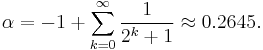
In the worst case, merge sort does about 39% fewer comparisons than quicksort does in the average case; merge sort always makes fewer comparisons than quicksort, except in extremely rare cases, when they tie, where merge sort's worst case is found simultaneously with quicksort's best case. In terms of moves, merge sort's worst case complexity is O(n log n)—the same complexity as quicksort's best case, and merge sort's best case takes about half as many iterations as the worst case.
Recursive implementations of merge sort make 2n − 1 method calls in the worst case, compared to quicksort's n, thus merge sort has roughly twice as much recursive overhead as quicksort. However, iterative, non-recursive implementations of merge sort, avoiding method call overhead, are not difficult to code. Merge sort's most common implementation does not sort in place; therefore, the memory size of the input must be allocated for the sorted output to be stored in (see below for versions that need only n/2 extra spaces).
Stable sorting in-place is possible but is more complicated, and usually a bit slower, even if the algorithm also runs in O(n log n) time (Katajainen, Pasanen & Teuhola 1996). One way to sort in-place is to merge the blocks recursively.[4] Like the standard merge sort, in-place merge sort is also a stable sort. Stable sorting of linked lists is simpler. In this case the algorithm does not use more space than that the already used by the list representation, but the O(log(k)) used for the recursion trace.
Merge sort is more efficient than quick sort for some types of lists if the data to be sorted can only be efficiently accessed sequentially, and is thus popular in languages such as Lisp, where sequentially accessed data structures are very common. Unlike some (efficient) implementations of quicksort, merge sort is a stable sort as long as the merge operation is implemented properly.
Merge sort also has some demerits. One is its use of 2n locations; the additional n locations are commonly used because merging two sorted sets in place is more complicated and would need more comparisons and move operations. But despite the use of this space the algorithm still does a lot of work: The contents of m are first copied into left and right and later into the list result on each invocation of merge_sort (variable names according to the pseudocode above). An alternative to this copying is to associate a new field of information with each key (the elements in m are called keys). This field will be used to link the keys and any associated information together in a sorted list (a key and its related information is called a record). Then the merging of the sorted lists proceeds by changing the link values; no records need to be moved at all. A field which contains only a link will generally be smaller than an entire record so less space will also be used.
Another alternative for reducing the space overhead to n/2 is to maintain left and right as a combined structure, copy only the left part of m into temporary space, and to direct the merge routine to place the merged output into m. With this version it is better to allocate the temporary space outside the merge routine, so that only one allocation is needed. The excessive copying mentioned in the previous paragraph is also mitigated, since the last pair of lines before the return result statement (function merge in the pseudo code above) become superfluous.
Merge sort can also be done with merging more than two sublists at a time, using the n-way merge algorithm. However, the number of operations is approximately the same. Consider merging k sublists at a time, where for simplicity k is a power of 2. The recurrence relation becomes T(n) = k T(n/k) + O(n log k). (The last part comes from the merge algorithm, which when implemented optimally using a heap or self-balancing binary search tree, takes O (log k) time per element.) If you take the recurrence relation for regular merge sort (T(n) = 2T(n/2) + O(n)) and expand it out log2k times, you get the same recurrence relation. This is true even if k is not a constant.
Use with tape drives
An external merge sort is practical to run using tape drives as input and output devices. It requires very little memory, and the memory required does not depend on the number of records.
For the same reason it is also useful for sorting data on disk that is too large to fit entirely into primary memory. On tape drives that can run both backwards and forwards, merge passes can be run in both directions, avoiding rewind time.
If you have four tape drives, it works as follows:
- Divide the data to be sorted in half and put half on each of two tapes
- Merge individual pairs of records from the two tapes; write two-record chunks alternately to each of the two output tapes
- Merge the two-record chunks from the two output tapes into four-record chunks; write these alternately to the original two input tapes
- Merge the four-record chunks into eight-record chunks; write these alternately to the original two output tapes
- Repeat until you have one chunk containing all the data, sorted --- that is, for log n passes, where n is the number of records.
For almost-sorted data on tape, a bottom-up "natural merge sort" variant of this algorithm is popular.
The bottom-up "natural merge sort" merges whatever "runs" of in-order records are already in the data. In the worst case (reversed data), "natural merge sort" performs the same as the above—it merges individual records into 2-record chunks, then 2-record chunks into 4-record chunks, etc. In the best case (already mostly-sorted data), "natural merge sort" merges large already-sorted chunks into even larger chunks, hopefully finishing in fewer than log n passes.
In a simple pseudocode form, the "natural merge sort" algorithm could look something like this:
 # Original data is on the input tape; the other tapes are blank
 function merge_sort(input_tape, output_tape, scratch_tape_C, scratch_tape_D)
     while any records remain on the input_tape
         while any records remain on the input_tape
             merge( input_tape, output_tape, scratch_tape_C)
             merge( input_tape, output_tape, scratch_tape_D)
         while any records remain on C or D
             merge( scratch_tape_C, scratch_tape_D, output_tape)
             merge( scratch_tape_C, scratch_tape_D, input_tape)
 # take the next sorted run from the input tapes, and merge into the single given output_tape.
 # tapes are scanned linearly.
 # tape[next] gives the record currently under the read head of that tape.
 # tape[current] gives the record previously under the read head of that tape.
 # (Generally both tape[current] and tape[previous] are buffered in RAM ...)
 function merge(left[], right[], output_tape[])
     do
        if left[current] ≤ right[current]
            append left[current] to output_tape
            read next record from left tape
        else
            append right[current] to output_tape
            read next record from right tape
    while left[current] < left[next] and right[current] < right[next]
    if left[current] < left[next]
        append current_left_record to output_tape
    if right[current] < right[next]
        append current_right_record to output_tape
    return
Either form of merge sort can be generalized to any number of tapes.
A more sophisticated merge sort is the polyphase merge sort.
Optimizing merge sort
On modern computers, locality of reference can be of paramount importance in software optimization, because multilevel memory hierarchies are used. Cache-aware versions of the merge sort algorithm, whose operations have been specifically chosen to minimize the movement of pages in and out of a machine's memory cache, have been proposed. For example, the tiled merge sort algorithm stops partitioning subarrays when subarrays of size S are reached, where S is the number of data items fitting into a CPU's cache. Each of these subarrays is sorted with an in-place sorting algorithm, to discourage memory swaps, and normal merge sort is then completed in the standard recursive fashion. This algorithm has demonstrated better performance on machines that benefit from cache optimization. (LaMarca & Ladner 1997)
Kronrod (1969) suggested an alternative version of merge sort that uses constant additional space. This algorithm was later refined. (Katajainen, Pasanen & Teuhola 1996).
Also, many applications of external sorting use a form of merge sorting where the input get split up to a higher number of sublists, ideally to a number for which merging them still makes the currently processed set of pages fit into main memory.
Parallel processing
Merge sort parallelizes well due to use of divide-and-conquer method. A parallel implementation is shown in pseudo-code in the third edition of Cormen, Leiserson, and Stein's Introduction to Algorithms.[5] This algorithm uses parallel merge algorithm to not only parallelize the recursive division of the array, but also the merge operation. It performs well in practice when combined with a fast stable sequential sort, such as insertion sort, and a fast sequential merge as a base case for merging small arrays.[6] Merge sort was one of the first sorting algorithms where optimal speed up was achieved, with Richard Cole using a clever subsampling algorithm to ensure O(1) merge.[7] Other sophisticated parallel sorting algorithms can achieve the same or better time bounds with a lower constant. For example, in 1991 David Powers described a parallelized quicksort (and a related radix sort) that can operate in O(log n) time on a CRCW PRAM with n processors by performing partitioning implicitly.[8]
Comparison with other sort algorithms
Although heapsort has the same time bounds as merge sort, it requires only Θ(1) auxiliary space instead of merge sort's Θ(n), and is often faster in practical implementations. On typical modern architectures, efficient quicksort implementations generally outperform mergesort for sorting RAM-based arrays. On the other hand, merge sort is a stable sort, parallelizes better, and is more efficient at handling slow-to-access sequential media. Merge sort is often the best choice for sorting a linked list: in this situation it is relatively easy to implement a merge sort in such a way that it requires only Θ(1) extra space, and the slow random-access performance of a linked list makes some other algorithms (such as quicksort) perform poorly, and others (such as heapsort) completely impossible.
As of Perl 5.8, merge sort is its default sorting algorithm (it was quicksort in previous versions of Perl). In Java, the Arrays.sort() methods use merge sort or a tuned quicksort depending on the datatypes and for implementation efficiency switch to insertion sort when fewer than seven array elements are being sorted.[9] Python uses timsort, another tuned hybrid of merge sort and insertion sort, which will also become the standard sort algorithm for Java SE 7.[10]
Utility in online sorting
Merge sort's merge operation is useful in online sorting, where the list to be sorted is received a piece at a time, instead of all at the beginning. In this application, we sort each new piece that is received using any sorting algorithm, and then merge it into our sorted list so far using the merge operation. However, this approach can be expensive in time and space if the received pieces are small compared to the sorted list — a better approach in this case is to insert elements into a binary search tree as they are received.
Notes
- ^ Knuth (1998, p. 158)
- ^ Jyrki Katajainen and Jesper Larsson Träff (1997). A meticulous analysis of mergesort programs.
- ^ The worst case number given here does not agree with that given in Knuth's Art of Computer Programming, Vol 3. The discrepancy is due to Knuth analyzing a variant implementation of merge sort that is slightly sub-optimal
- ^ A Java implementation of in-place stable merge sort
- ^ Cormen et al. 2009, p. 803
- ^ V. J. Duvanenko, "Parallel Merge Sort", Dr. Dobb's Journal, March 2011
- ^ Cole, Richard (August 1988), "Parallel merge sort", SIAM J. Comput. 17 (4): 770–785
- ^ Powers, David M. W. Parallelized Quicksort and Radixsort with Optimal Speedup, Proceedings of International Conference on Parallel Computing Technologies. Novosibirsk. 1991.
- ^ OpenJDK Subversion
- ^ http://hg.openjdk.java.net/jdk7/tl/jdk/rev/bfd7abda8f79
References
- Cormen, Thomas H.; Leiserson, Charles E., Rivest, Ronald L., Stein, Clifford (2009) [1990]. Introduction to Algorithms (3rd ed.). MIT Press and McGraw-Hill. ISBN 0-262-03384-4.
- Katajainen, Jyrki; Pasanen, Tomi; Teuhola, Jukka (1996). "Practical in-place mergesort". Nordic Journal of Computing 3: pp. 27–40. ISSN 1236-6064. http://www.diku.dk/hjemmesider/ansatte/jyrki/Paper/mergesort_NJC.ps. Retrieved 2009-04-04. Also Practical In-Place Mergesort. Also [1]
- Knuth, Donald (1998). "Section 5.2.4: Sorting by Merging". Sorting and Searching. The Art of Computer Programming. 3 (2nd ed.). Addison-Wesley. pp. 158–168. ISBN 0-201-89685-0.
- Kronrod, M. A. (1969). "Optimal ordering algorithm without operational field". Soviet Mathematics - Doklady 10: pp. 744
- LaMarca, A.; Ladner, R. E. (1997). "The influence of caches on the performance of sorting". Proc. 8th Ann. ACM-SIAM Symp. on Discrete Algorithms (SODA97): 370–379
- Sun Microsystems, Inc.. "Arrays API". http://java.sun.com/javase/6/docs/api/java/util/Arrays.html. Retrieved 2007-11-19.
- Sun Microsystems, Inc.. "java.util.Arrays.java". https://openjdk.dev.java.net/source/browse/openjdk/jdk/trunk/jdk/src/share/classes/java/util/Arrays.java?view=markup. Retrieved 2007-11-19.
External links
- Animated Sorting Algorithms: Merge Sort – graphical demonstration and discussion of array-based merge sort
- Dictionary of Algorithms and Data Structures: Merge sort
|
||||||||||||||||||||||||||||||||