Kochen–Specker theorem
In quantum mechanics, the Kochen–Specker (KS) theorem[1] is a "no go" theorem proved by Simon B. Kochen and Ernst Specker in 1967. It places certain constraints on the permissible types of hidden variable theories which try to explain the apparent randomness of quantum mechanics as a deterministic model featuring hidden states. The theorem is a complement to Bell's theorem.
The theorem proves that there is a contradiction between two basic assumptions of the hidden variable theories intended to reproduce the results of quantum mechanics: that all hidden variables corresponding to quantum mechanical observables have definite values at any given time, and that the values of those variables are intrinsic and independent of the device used to measure them. The contradiction is caused by the fact that quantum mechanical observables need not be commutative, making it impossible to embed the algebra of these observables in a commutative algebra, assumed to represent the classical structure of the hidden variables theory.
The Kochen–Specker proof demonstrates the impossibility of Einstein's assumption, made in the famous Einstein–Podolsky–Rosen paper[2], that quantum mechanical observables represent 'elements of physical reality'. More generally, the theorem excludes hidden variable theories that require elements of physical reality to be non-contextual (i.e. independent of the measurement arrangement).
Contents |
History
The KS theorem is an important step in the debate on the (in)completeness of quantum mechanics, boosted in 1935 by the criticism in the EPR paper of the Copenhagen assumption of completeness, creating the so-called EPR paradox. This paradox is derived from the assumption that a quantum mechanical measurement result is generated in a deterministic way as a consequence of the existence of an element of physical reality assumed to be present before the measurement as a property of the microscopic object. In the EPR paper it was assumed that the measured value of a quantum mechanical observable can play the role of such an element of physical reality. As a consequence of this metaphysical supposition the EPR criticism was not taken very seriously by the majority of the physics community. Moreover, in his answer[3] Bohr had pointed to an ambiguity in the EPR paper, to the effect that it assumes the value of a quantum mechanical observable is non-contextual (i.e. is independent of the measurement arrangement). Taking into account the contextuality stemming from the measurement arrangement would, according to Bohr, make obsolete the EPR reasoning. It was subsequently observed by Einstein[4] that Bohr's reliance on contextuality implies nonlocality ("spooky action at a distance"), and that, in consequence, one would have to accept incompleteness if one wanted to avoid nonlocality.
In the 1950s and '60s two lines of development were open for those not averse to metaphysics, both lines improving on a "no go" theorem presented by von Neumann[5], purporting to prove the impossibility of the hidden variable theories yielding the same results as quantum mechanics. First, Bohm developed an interpretation of quantum mechanics, generally accepted as a hidden variable theory underpinning quantum mechanics. The nonlocality of Bohm's theory induced Bell to assume that quantum reality is nonlocal, and that probably only local hidden variable theories are in disagreement with quantum mechanics. More importantly, Bell managed to lift the problem from the level of metaphysics to physics by deriving an inequality, the Bell inequality, that is capable of being experimentally tested.
A second line is the Kochen–Specker one. The essential difference from Bell's approach is that the possibility of underpinning quantum mechanics by a hidden variable theory is dealt with independently of any reference to nonlocality. Although contextuality plays an important part, there is no implication of nonlocality because the proof refers to observables belonging to one single object, to be measured in one and the same region of space. Contextuality is related here with incompatibility of quantum mechanical observables, incompatibility being associated with mutual exclusiveness of measurement arrangements.
Considerably simpler proofs than the Kochen–Specker one were given later, amongst others, by Mermin[6] and by Peres[7].
The KS theorem
The KS theorem explores whether it is possible to embed the set of quantum mechanical observables into a set of classical quantities, notwithstanding that all classical quantities are mutually compatible. The first observation made in the Kochen–Specker paper, is that this is possible in a trivial way, viz. by ignoring the algebraic structure of the set of quantum mechanical observables. Indeed, let pA(ak) be the probability that observable A has value ak, then the product ΠApA(ak), taken over all possible observables A, is a valid joint probability distribution, yielding all probabilities of quantum mechanical observables by taking marginals. Kochen and Specker note that this joint probability distribution is not acceptable, however, since it ignores all correlations between the observables. Thus, in quantum mechanics A2 has value ak2 if A has value ak, implying that the values of A and A2 are highly correlated.
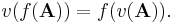
More generally it is required by Kochen and Specker that for an arbitrary function f the value  of observable
  satisfies
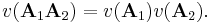
If A1 and A2 are compatible (commeasurable) observables, then, by the same token, we should have the following two equalities

 and
and  real, and
The first of the latter two equalities is a considerable weakening compared to von Neumann's assumption that this equality should hold independently of whether A1 and A2 are compatible or incompatible. Kochen and Specker were capable of proving that a value assignment is not possible even on the basis of these weaker assumptions. In order to do so they restricted the observables to a special class, viz. so-called yes-no observables, having only values 0 and 1, corresponding to projection operators on the eigenvectors of certain orthogonal bases of a Hilbert space.
Restricting themselves to a three-dimensional Hilbert space, they were able to find a set of 117 such projection operators, not allowing to attribute to each of them in an unambiguous way either value 0 or 1. Instead of the rather involved proof by Kochen and Specker it is more illuminating to reproduce here one of the much simpler proofs given much later, which employs a lower number of projection operators by considering a four-dimensional Hilbert space. It turns out that it is possible to obtain a similar result on the basis of a set of only 18 projection operators. The method also works in an eight dimensional Hilbert Space. [8]
In order to do so it is sufficient to realize that, if u1, u2, u3 and u4 are the four orthogonal vectors of an orthogonal basis in the four-dimensional Hilbert space, then the projection operators P1, P2, P3, P4 on these vectors are all mutually commuting (and, hence, correspond to compatible observables, allowing a simultaneous attribution of values 0 or 1). Since

it follows that

But, since

it follows from  0 or 1,
  , that out of the four values
  , one must be 1 while the other three must be 0.
Cabello[9], extending an argument developed by Kernaghan [10] considered 9 orthogonal bases, each basis corresponding to a column of the following table, in which the basis vectors are explicitly displayed. The bases are chosen in such a way that each has a vector in common with one other basis (indicated in the table by equal colours), thus establishing certain correlations between the 36 corresponding yes-no observables.
| u1 | (0, 0, 0, 1) | (0, 0, 0, 1) | (1, –1, 1, –1) | (1, –1, 1, –1) | (0, 0, 1, 0) | (1, –1, –1, 1) | (1, 1, –1, 1) | (1, 1, –1, 1) | (1, 1, 1, –1) |
| u2 | (0, 0, 1, 0) | (0, 1, 0, 0) | (1, –1, –1, 1) | (1, 1, 1, 1) | (0, 1, 0, 0) | (1, 1, 1, 1) | (1, 1, 1, –1) | (–1, 1, 1, 1) | (–1, 1, 1, 1) |
| u3 | (1, 1, 0, 0) | (1, 0, 1, 0) | (1, 1, 0, 0) | (1, 0, –1, 0) | (1, 0, 0, 1) | (1, 0, 0, –1) | (1, –1, 0, 0) | (1, 0, 1, 0) | (1, 0, 0, 1) |
| u4 | (1, –1, 0, 0) | (1, 0, –1, 0) | (0, 0, 1, 1) | (0, 1, 0, –1) | (1, 0, 0, –1) | (0, 1, –1, 0) | (0, 0, 1, 1) | (0, 1, 0, –1) | (0, 1, –1, 0) |
Now the "no go" theorem easily follows by making sure that it is impossible to distribute the four numbers 1,0,0,0 over the four rows of each column, such that equally coloured compartments contain equal numbers. Another way to see the theorem, using the approach by Kernaghan, is to recognize that a contradiction is implied between the odd number of bases and the even number of occurrences of the observables.
Remarks on the KS theorem
1. Contextuality
In the Kochen–Specker paper the possibility is discussed that the value attribution  may be context-dependent, i.e. observables corresponding to equal vectors in different columns of the table need not have equal values because different columns correspond to different measurement arrangements. Since subquantum reality (as described by the hidden variable theory) may be dependent on the measurement context, it is possible that relations between quantum mechanical observables and hidden variables are just homomorphic rather than isomorphic. This would make obsolete the requirement of a context-independent value attribution. Hence, the KS theorem does only exclude noncontextual hidden variable theories. The possibility of contextuality has given rise to the so-called modal interpretations of quantum mechanics.
2. Different levels of description
By the KS theorem the impossibility is proven of Einstein's assumption that an element of physical reality is represented by a value of a quantum mechanical observable. The question may be asked whether this is a very shocking result. The value of a quantum mechanical observable refers in the first place to the final position of the pointer of a measuring instrument, which comes into being only during the measurement, and which, for this reason, cannot play the role of an element of physical reality. Elements of physical reality, if existing, would seem to need a subquantum (hidden variable) theory for their description rather than quantum mechanics. In later publications[11] the Bell inequalities are discussed on the basis of hidden variable theories in which the hidden variable is supposed to refer to a subquantum property of the microscopic object different from the value of a quantum mechanical observable. This opens up the possibility of distinguishing different levels of reality described by different theories, which, incidentally, had already been practised by Louis de Broglie. For such more general theories the KS theorem is applicable only if the measurement is assumed to be a faithful one, in the sense that there is a deterministic relation between a subquantum element of physical reality and the value of the observable found on measurement. The existence or nonexistence of such subquantum elements of physical reality is not touched by the KS theorem. As an example, recent experiments on bouncing drops on a vibrating bath, by Y. Couder and collaborators, reproduce many features of quantum mechanics[12][13] [14] [15] [16][17] [18]. In this case, the subquantum elements of physical reality are linked to the specifics of the hydrodynamics of bouncing drops on a vibrating bath (linked to the Faraday wave instability phenomenology [19]). At the level that reproduces features of quantum mechanics, measurement are not deterministic since they depend on the stochastic nature of the non-linear dynamics of the subquantum elements. The experiments are indeed interpreted in the framework of De Broglie–Bohm theory of pilot waves.
Notes
- ^ S. Kochen and E.P. Specker, "The problem of hidden variables in quantum mechanics", Journal of Mathematics and Mechanics 17, 59–87 (1967).
- ^ A. Einstein, B. Podolsky and N. Rosen, "Can quantum-mechanical description of physical reality be considered complete?" Phys. Rev. 47, 777–780 (1935).
- ^ N. Bohr, "Can quantum-mechanical description of physical reality be considered complete?" Phys. Rev. 48, 696–702 (1935).
- ^ A. Einstein, "Quanten-Mechanik und Wirklichkeit", Dialectica 2, 320 (1948).
- ^ J. von Neumann, Mathematische Grundlagen der Quantenmechanik, Springer, Berlin, 1932; English translation: Mathematical foundations of quantum mechanics, Princeton Univ. Press, 1955, Chapter IV.1,2.
- ^ N.D. Mermin, "What's wrong with these elements of reality?" Physics Today, 43, Issue 6, 9–11 (1990); N.D. Mermin, "Simple unified form for the major no-hidden-variables theorems", Phys. Rev. Lett. 65, 3373 (1990).
- ^ A. Peres, "Two simple proofs of the Kochen–Specker theorem", J. Phys. A: Math. Gen. 24, L175–L178 (1991).
- ^ M. Kernaghan and A. Peres, Phys. Lett. A 198 (1995) 1–5.
- ^ A. Cabello, "A proof with 18 vectors of the Bell–Kochen–Specker theorem", in: M. Ferrero and A. van der Merwe (eds.), New Developments on Fundamental Problems in Quantum Physics, Kluwer Academic, Dordrecht, Holland, 1997, 59–62; Adan Cabello, Jose M. Estebaranz, Guillermo Garcia Alcaine, "Bell–Kochen–Specker theorem: A proof with 18 vectors", quant-ph/9706009v1, http://arxiv.org/abs/quant-ph/9706009v1
- ^ M. Kernaghan, J. Phys. A 27 (1994) L829.
- ^ e.g. J.F. Clauser and M.A. Horne, "Experimental consequences of objective local theories", Physical Review D 10, 526–535 (1974).
- ^ John W. M. Bush, Quantum mechanics writ large, PNAS 107, 17455–17456 (2010). [1]
- ^ Protière S., Boudaoud A., Couder Y. Particle wave association on a fluid interface J. Fluid Mech. 554, 85-108 (2006).
- ^ Couder Y., Protière S., Fort E., Boudaoud A. Dynamical phenomena: Walking and orbiting droplets Nature 437, 208 (2005).
- ^ Couder Y., Fort E. Single-particle diffraction and interference at a macroscopic scale Phys. Rev. Lett. 97, 154101-1–154101-4 (2006).
- ^ Eddi A., Fort E., Moisy F., Couder Y. Unpredictable tunneling of a classical wave-particle association Phys. Rev. Lett. 102, 240401-1–240401-4 (2009).
- ^ Eddi A., Decelle A., Fort E., Couder Y. Archimedean lattices in the bound states of wave interacting particles Europhys. Lett. 87, 56002-p1–56002-p6 (2009).
- ^ Fort E., Eddi A., Boudaoud A., Moukhtar J., Couder Y. Path-memory induced quantization of classical orbits Proc. Natl. Acad. Sci. USA 107, 17515–17520 (2010).
- ^ Couder Y., Fort E., Gautier C.H., Boudaoud A. From bouncing to floating: Noncoalescence of drops on a fluid bath Phys. Rev. Lett. 94 177801-1–177801-4 (2005).
External links
- Carsten Held, The Kochen–Specker Theorem, Stanford Encyclopedia of Philosophy *[2]
- Kochen-Specker theorem on arxiv.org
- S. Kochen and E. P. Specker, The problem of hidden variables in quantum mechanics, Full text [3]