Karush–Kuhn–Tucker conditions

In mathematics, the Karush–Kuhn–Tucker (KKT) conditions (also known as the Kuhn–Tucker conditions) are necessary for a solution in nonlinear programming to be optimal, provided that some regularity conditions are satisfied. Allowing inequality constraints, the KKT approach to nonlinear programming generalizes the method of Lagrange multipliers, which allows only equality constraints. The KKT conditions were originally named after Harold W. Kuhn, and Albert W. Tucker, who first published the conditions.^[1] Later scholars discovered that the necessary conditions for this problem had been stated by William Karush in his master's thesis.^[2]^[3]

1 Nonlinear optimization problem
2 Necessary conditions
3 Regularity conditions (or constraint qualifications)
4 Sufficient conditions
5 Value function
6 Generalizations
7 See also
8 References
9 Further reading

Nonlinear optimization problem

We consider the following nonlinear optimization problem:

$\text{Minimize }\; f(x)$

$\text{subject to: }\$

$g_i(x) \le 0 , h_j(x) = 0$

where x is the optimization variable, $f( \cdot )$ is the objective or cost function, $g_i (\cdot)\ (i = 1, \ldots,m)$ are the inequality constraint functions, and $h_j (\cdot)\ (j = 1,\ldots,l)$ are the equality constraint functions. The number of inequality and equality constraints are denoted m and l, respectively.

Necessary conditions

Suppose that the objective function $f�: \mathbb{R}^n \rightarrow \mathbb{R}$ and the constraint functions $g_i�: \,\!\mathbb{R}^n \rightarrow \mathbb{R}$ and $h_j�: \,\!\mathbb{R}^n \rightarrow \mathbb{R}$ are continuously differentiable at a point $x^*$ . If $x^*$ is a local minimum that satisfies some regularity conditions (see below), then there exist constants 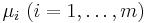$\mu_i\ (i = 1,\ldots,m)$ and $\lambda_j\ (j = 1,\ldots,l)$ , called KKT multipliers, such that

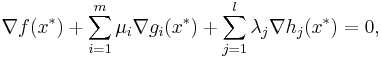
Stationarity: $\nabla f(x^*) %2B \sum_{i=1}^m \mu_i \nabla g_i(x^*) %2B \sum_{j=1}^l \lambda_j \nabla h_j(x^*) = 0,$

Primal feasibility: $g_i(x^*) \le 0, \mbox{ for all } i = 1, \ldots, m$; $h_j(x^*) = 0, \mbox{ for all } j = 1, \ldots, l \,\!$

Dual feasibility: $\mu_i \ge 0, \mbox{ for all } i = 1, \ldots, m$

Complementary slackness: $\mu_i g_i (x^*) = 0, \mbox{for all}\; i = 1,\ldots,m.$

In the particular case $m=0$ , i.e., when there are no inequality constraints, the KKT conditions turn into the Lagrange conditions, and the KKT multipliers are called Lagrange multipliers.

Regularity conditions (or constraint qualifications)

In order for a minimum point $x^*$ to satisfy the above KKT conditions, it should satisfy some regularity condition, the most used ones are listed below:

Linear independence constraint qualification (LICQ): the gradients of the active inequality constraints and the gradients of the equality constraints are linearly independent at $x^*$ .
Mangasarian–Fromovitz constraint qualification (MFCQ): the gradients of the active inequality constraints and the gradients of the equality constraints are positive-linearly independent at $x^*$ .
Constant rank constraint qualification (CRCQ): for each subset of the gradients of the active inequality constraints and the gradients of the equality constraints the rank at a vicinity of $x^*$ is constant.
Constant positive linear dependence constraint qualification (CPLD): for each subset of the gradients of the active inequality constraints and the gradients of the equality constraints, if it is positive-linear dependent at $x^*$ then it is positive-linear dependent at a vicinity of $x^*$ .
Quasi-normality constraint qualification (QNCQ): if the gradients of the active inequality constraints and the gradients of the equality constraints are positive-linearly independent at $x^*$ with associated multipliers $\lambda_i$ for equalities and $\mu_j$ for inequalities, then there is no sequence $x_k\to x^*$ such that 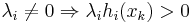$\lambda_i \neq 0 \Rightarrow \lambda_i h_i(x_k)>0$ and $\mu_j \neq 0 \Rightarrow \mu_j g_j(x_k)>0$ .
Slater condition: for a convex problem, there exists a point $x$ such that $h(x)=0$ and $g_i(x) < 0$ for all $i$ active in $x^*$ .
Linearity constraints: If $f$ and $g$ are affine functions, then no other condition is needed to assure that the minimum point is KKT.

( $v_1,\ldots,v_n$ ) is positive-linear dependent if there exists $a_1\geq 0,\ldots,a_n\geq 0$ not all zero such that $a_1v_1%2B\ldots%2Ba_nv_n=0$ .

It can be shown that LICQ⇒MFCQ⇒CPLD⇒QNCQ, LICQ⇒CRCQ⇒CPLD⇒QNCQ (and the converses are not true), although MFCQ is not equivalent to CRCQ^[4] . In practice weaker constraint qualifications are preferred since they provide stronger optimality conditions.

Sufficient conditions

In some cases, the necessary conditions are also sufficient for optimality. In general, the necessary conditions are not sufficient for optimality and additional information is necessary, such as the Second Order Sufficient Conditions (SOSC). For smooth functions, SOSC involve the second derivatives, which explains its name.

The necessary conditions are sufficient for optimality if the objective function $f$ and the inequality constraints $g_j$ are continuously differentiable convex functions and the equality constraints $h_i$ are affine functions.

It was shown by Martin in 1985^[5] that the broader class of functions in which KKT conditions guarantees global optimality are the so called Type 1 invex functions.^[6]

Value function

If we reconsider the optimization problem as a maximization problem with constant inequality constraints,

$\text{Maximize }\; f(x)$

$\text{subject to: }\$

$g_i(x) \le a_i , h_j(x) = 0.$

The value function is defined as:

$V(a_1, \ldots a_n) = \sup\limits_x f(x)$

$\text{subject to: }\$

$g_i(x) \le a_i , h_j(x) = 0$

$j\in\{1,\ldots l\}, i\in\{1,\ldots,m\}.$

(So the domain of V is $\{a \in \mathbb{R}^m | \text{for some }x\in X, g_i(x) \leq a_i, i \in \{1,\ldots,m\}.$ )

Given this definition, each coefficient, $\mu_i$ , is the rate at which the value function increases as $a_i$ increases. Thus if each $a_i$ is interpreted as a resource constraint, the coefficients tell you how much increasing a resource will increase the optimum value of our function f. This interpretation is especially important in economics and is used, for instance, in utility maximization problems.

Generalizations

With an extra constant multiplier $\mu_0$ , which may be zero, in front of $\nabla f(x^*)$ the KKT stationarity conditions turn into

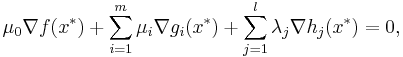
$\mu_0 \nabla f(x^*) %2B \sum_{i=1}^m \mu_i \nabla g_i(x^*) %2B \sum_{j=1}^l \lambda_j \nabla h_j(x^*) = 0,$

which are called the Fritz John conditions.

The KKT conditions belong to a wider class of the First Order Necessary Conditions (FONC), which allow for non-smooth functions using subderivatives.

References

^ Kuhn, H. W.; Tucker, A. W. (1951). "Nonlinear programming". Proceedings of 2nd Berkeley Symposium. Berkeley: University of California Press. pp. 481–492. http://projecteuclid.org/euclid.bsmsp/1200500249. MR 47303
^ W. Karush (1939). Minima of Functions of Several Variables with Inequalities as Side Constraints. M.Sc. Dissertation. Dept. of Mathematics, Univ. of Chicago, Chicago, Illinois.
^ Kjeldsen, Tinne Hoff. "A contextualized historical analysis of the Kuhn-Tucker theorem in nonlinear programming: the impact of World War II". Historia Math. 27 (2000), no. 4, 331–361. MR 1800317
^ Rodrigo Eustaquio, Elizabeth Karas, and Ademir Ribeiro. Constraint Qualification for Nonlinear Programming (Technical report). Federal University of Parana. http://pessoal.utfpr.edu.br/eustaquio/arquivos/kkt.pdf.
^ Martin, D. H. (1985). "The essence of invexity". J. Optim. Theory Appl., 47. pp. 65–76.
^ M.A. Hanson, Invexity and the Kuhn-Tucker Theorem, J. Math. Anal. Appl. vol. 236, pp. 594–604 (1999)

Karush–Kuhn–Tucker conditions

Contents

Nonlinear optimization problem

Necessary conditions

Regularity conditions (or constraint qualifications)

Sufficient conditions

Value function

Generalizations

See also

References

Further reading