Incomplete gamma function
In mathematics, the gamma function is defined by a definite integral. The incomplete gamma function is defined as an integral function of the same integrand. There are two varieties of the incomplete gamma function: the upper incomplete gamma function is for the case that the lower limit of integration is variable (i.e. where the "upper" limit is fixed), and the lower incomplete gamma function can vary the upper limit of integration.
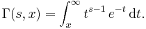
The upper incomplete gamma function is defined as:
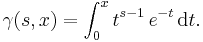
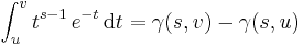
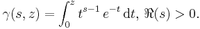
The lower incomplete gamma function is defined as:
Contents |
Properties
In both cases s is a complex parameter, such that the real part of s is positive.
By integration by parts we find the recurrence relations

and conversely

Since the ordinary gamma function is defined as
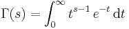
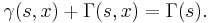
we have
Continuation to complex values
The lower incomplete gamma and the upper incomplete gamma function, as defined above for real positive s and x, can be developed into holomorphic functions, with respect both to x and s, defined for almost all combinations of complex x and s.[1]. Complex analysis shows how properties of the real incomplete gamma functions extend to their holomorphic counterparts.
Lower Incomplete Gamma Function
Holomorphic Extension
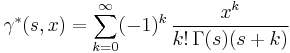
Repeated application of the recurrence relation for the lower incomplete gamma function leads to the power series expansion: [3]
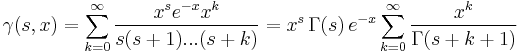
Given the rapid growth in absolute value of  when k → ∞, and the fact that the reciprocal of
  is an entire function, the coefficients in the rightmost sum are well-defined, and locally the sum converges uniformly for all complex s and x. By a theorem of Weierstraß,[2] the limiting function, sometimes denoted as
  ,
,
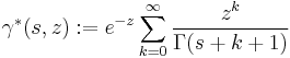
is entire with respect to both z (for fixed s) and s (for fixed z) [5], and, thus, holomorphic on ℂ×ℂ by Hartog's theorem[6]. Hence, the following decomposition
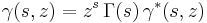 [7],
[7],
extends the real lower incomplete gamma function as a holomorphic function, both jointly and separately in z and s. It follows from the properties of  and the
  -function, that the first two factors capture the singularities of
  (z = 0 and s a non-positive integer), whereas the last factor contributes to its zeros.
Branches
In particular, the factor causes to be multi-valued for s not an integer. This complication is often overcome by cutting the image of , for fixed s, (usually) along the negative real axis into separate, single-valued branches, and then restricting oneself to the principal branch corresponding to that of . Values from other branches can be derived by multiplication by  [8], k an integer. (For another view on these phenomena see Riemann surfaces).
Behavior near Branch Point
The decomposition above further shows, that behaves near z = 0 asymptotically like:

For positive real x, y and s,  , when (x, y) → (0, s). This seems to justify setting
  for real s > 0. However, matters are somewhat different in the complex realm. Only if (a) the real part of s is positive, and (b) values from just a finite set of branches of
  are taken, then is guaranteed to converge to zero as (u, v) → (0, s), and so does
  . A single branch of naturally fulfills (b), so for s with positive real part is a continuous limit there. Also note that such a continuation is by no means an analytic one.
Algebraic Relations
All algebraic relations and differential equations observed by the real  hold for its holomorphic counterpart as well. This is a consequence of the identity theorem [9], stating that equations between holomorphic functions valid on a real interval, hold everywhere. In particular, the recurrence relation [10] and
 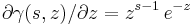 [11] are preserved on corresponding branches.
Integral Representation
The last relation tells us, that, for fixed s, is a primitive or antiderivative of the holomorphic function  . Consequently [12], for any complex u, v ≠ 0,
holds, as long as the path of integration does not wind around the singular branch point 0. If the image of the path is entirely contained in the interior of a single branch of the integrand, and the real part of s is positive, then the limit  → 0 for u → 0 applies, finally arriving at the complex integral definition of
Any path of integration containing 0 only at its beginning, and never crossing or touching the negative real line, is valid here, for example, the straight line connecting 0 and z. If z is a negative real, some technical adjustments are required to guarantee the result is from the correct branch.
Overview
is:
- entire in z for fixed, positive integral s;
- multi-valued holomorphic in z for fixed s not an integer, with a branch point at z = 0;
- on each branch meromorphic in s for fixed z ≠ 0, with simple poles at non-positive integers s.
Upper Incomplete Gamma Function
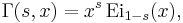
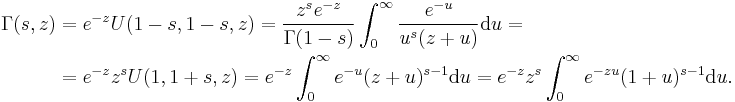
As for the upper incomplete gamma function, a holomorphic extension, with respect to z or s, is given by
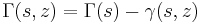
at points (s, z), where the right hand side exists. Since is multi-valued, the same holds for , but a restriction to principal values only yields the single-valued principal branch of .
When s is a non-positive integer in the above equation, neither part of the difference is defined, and a limiting process, here developed for s → 0, fills in the missing values. Complex analysis guarantees holomorphicity, because  proves to be bounded in a neighbourhood of that limit for a fixed z[15].
To determine the limit, the power series of at z = 0 turns out useful. When replacing  by its power series in the integral definition of , one obtains (assume x,s positive reals for now):

or
 . [16]
which, as a series representation of the entire function, converges for all complex x (and all complex s not a non-positive integer).
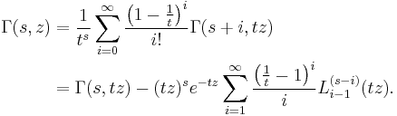
With its restriction to real values lifted, the series allows the expansion:

When s → 0:
 ,[3]
,[3]
( is the Euler-Mascheroni constant here), hence,

is the limiting function to the upper incomplete gamma function as s → 0, also known as  .[4]
.[4]
By way of the recurrence relation, values of  for positive integers n can be derived from this result, so the upper incomplete gamma function proves to exist and be holomorphic, with respect both to z and s, for all s and z ≠ 0.
is:
- entire in z for fixed, positive integral s;
- multi-valued holomorphic in z for fixed s not an integer, with a branch point at z = 0;
- =
 for s with positive real part and z = 0 (the limit when
  ), but this is a continuous extension, not an analytic one (does not hold for real s<0!);
 - on each branch entire in s for fixed z ≠ 0.
Special values
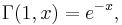
 if s is a positive integer,
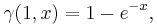
 if s is a positive
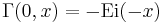 for
for 
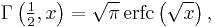
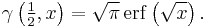
Here, Ei is the exponential integral, erf is the error function, and erfc is the complementary error function, erfc(x) = 1 − erf(x).
Asymptotic behavior
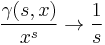 as
as 
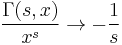 as
as  and
and 
 as
as 
 as
as
 as an asymptotic series where
  and
and  .[6]
.[6]
Evaluation formulae
The lower gamma function has the straight forward expansion
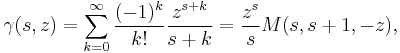
where M is Kummer's confluent hypergeometric function.
Connection with Kummer's confluent hypergeometric function
When the real part of z is positive,

where

has an infinite radius of convergence.
Again with confluent hypergeometric functions and employing Kummer's identity,
For the actual computation of numerical values, Gauss's continued fraction provides a useful expansion:
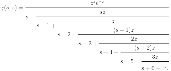
This continued fraction converges for all complex z, provided only that s is not a negative integer.
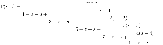
The upper gamma function has the continued fraction
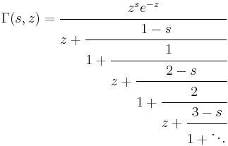
and
Multiplication theorem
The following multiplication theorem holds true:
Regularized Gamma functions and Poisson random variables
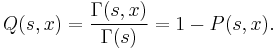
Two related functions are the regularized Gamma functions:
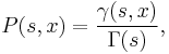
 is the cumulative distribution function for Gamma random variables with shape parameter
  and scale parameter 1.
When  is an integer,
  is the cumulative distribution function for Poisson random variables: If
  is a
is a  random variable then
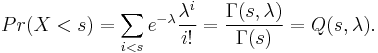
This formula can be derived by repeated integration by parts.
Derivatives
The derivative of the upper incomplete gamma function  with respect to x is well known. It is simply given by the integrand of its integral definition:
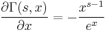
The derivative with respect to its first argument is given by[8]
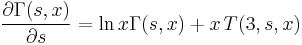
and the second derivative by
![\frac{\partial^2 \Gamma (s,x) }{\partial s^2} = \ln^2 x \Gamma (s,x) %2B 2 x[\ln x\,T(3,s,x) %2B T(4,s,x) ]](/2012-wikipedia_en_all_nopic_01_2012/I/7d0947440096f80c8a9f3977c2c74a45.png)
where the function  is a special case of the Meijer G-function
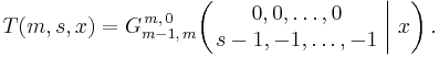
This particular special case has internal closure properties of its own because it can be used to express all successive derivatives. In general,

where
All such derivatives can be generated in succession from:

and
![\frac{\partial T (m,s,x) }{\partial x} = -\frac{1}{x} [T(m-1,s,x) %2B T(m,s,x)]](/2012-wikipedia_en_all_nopic_01_2012/I/c8dfc1eb606e4b32b18334c9eeb69095.png)
This function can be computed from its series representation valid for  ,
,
![T(m,s,z) = - \frac{(-1)^{m-1} }{(m-2)! } \frac{{\rm d}^{m-2} }{{\rm d}t^{m-2} } \left[\Gamma (s-t) z^{t-1}\right]\Big|_{t=0} %2B \sum_{n=0}^{\infty} \frac{(-1)^n z^{s-1%2Bn}}{n! (-s-n)^{m-1} }](/2012-wikipedia_en_all_nopic_01_2012/I/9c0a95062f351906edaa0b52f2fc9f57.png)
with the understanding that s is not a negative integer or zero. In such a case, one must use a limit. Results for  can be obtained by analytic continuation. Some special cases of this function can be simplified. For example,
  ,
,  , where
  is the Exponential integral. These derivatives and the function provide exact solutions to a number of integrals by repeated differentiation of the integral definition of the upper incomplete gamma function. [9] [10] For example,
This formula can be further inflated or generalized to a huge class of Laplace transforms and Mellin transforms. When combined with a computer algebra system, the exploitation of special functions provides a powerful method for solving definite integrals, in particular those encountered by practical engineering applications (see Symbolic integration for more details).
Indefinite and definite integrals
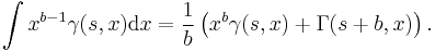
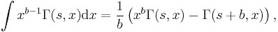
The following indefinite integrals are readily obtained using integration by parts:
The lower and the upper incomplete Gamma function are connected via the Fourier transform:
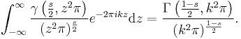
This follows, for example, by suitable specialization of (Gradshteyn & Ryzhik 1980, § 7.642).
Notes
- ^ DLMF, Incomplete Gamma functions, analytic continuation
- ^ [1] Theorem 3.9 on p.56
- ^ see last eq.
- ^ http://dlmf.nist.gov/8.4.E4
- ^ Weisstein, Eric W., "Incomplete Gamma Function" from MathWorld. (equation 2)
- ^ DLMF, Incomplete Gamma functions, 8.11(i)
- ^ Abramowitz and Stegun p. 263, 6.5.31
- ^ K.O. Geddes, M.L. Glasser, R.A. Moore and T.C. Scott, Evaluation of Classes of Definite Integrals Involving Elementary Functions via Differentiation of Special Functions, AAECC (Applicable Algebra in Engineering, Communication and Computing), vol. 1, (1990), pp. 149-165, [2]
- ^ Milgram, M. S. Milgram (1985). "The generalized integro-exponential function". Math. Comp. 44 (170): 443–458. doi:10.1090/S0025-5718-1985-0777276-4. MR0777276.
- ^ Mathar (2009). "Numerical Evaluation of the Oscillatory Integral over exp(i*pi*x)*x^(1/x) between 1 and infinity". arXiv:0912.3844 [math.CA]., App B
References
- Abramowitz, Milton; Stegun, Irene A., eds. (1965), "Chapter 6.5", Handbook of Mathematical Functions with Formulas, Graphs, and Mathematical Tables, New York: Dover, ISBN 978-0486612720, MR0167642, http://www.math.sfu.ca/~cbm/aands/page_.htm. "Incomplete Gamma function". http://www.math.sfu.ca/~cbm/aands/page_260.htm. §6.5.
- G. Arfken and H. Weber. Mathematical Methods for Physicists. Harcourt/Academic Press, 2000. (See Chapter 10.)
- DiDonato, Armido R.; Morris, Jr., Alfred H. (Dec. 1986). "Computation of the incomplete gamma function ratios and their inverse". ACM Transactions on Mathematical Software (TOMS) 12 (4): 377–393. doi:10.1145/22721.23109.
- DiDonato, Armido R.; Morris, Jr., Alfred H. (Sept. 1987). "ALGORITHM 654: FORTRAN subroutines for computing the incomplete gamma function ratios and their inverse". ACM Transactions on Mathematical Software (TOMS) 13 (3): 318–319. doi:10.1145/29380.214348. (See also Fortran 90 subroutines for ALGORITHM 654 )
- Gradshteyn, I.S.; Ryzhik, I.M. (1980). Tables of Integrals, Series, and Products (4th ed.). New York: Academic Press. ISBN 0-12-294760-6. (See Chapter 8.35.)
- Mathar, Richard J. (2004). "Numerical representation of the incomplete gamma function of complex-valued argument". Numerical Algorithms 36 (3): 247–264. doi:10.1023/B:NUMA.0000040063.91709.5. MR2091195.
- Paris, R. B. (2010), "Incomplete gamma function", in Olver, Frank W. J.; Lozier, Daniel M.; Boisvert, Ronald F. et al., NIST Handbook of Mathematical Functions, Cambridge University Press, ISBN 978-0521192255, MR2723248, http://dlmf.nist.gov/8
- Press, WH; Teukolsky, SA; Vetterling, WT; Flannery, BP (2007). "Section 6.2. Incomplete Gamma Function and Error Function". Numerical Recipes: The Art of Scientific Computing (3rd ed.). New York: Cambridge University Press. ISBN 978-0-521-88068-8. http://apps.nrbook.com/empanel/index.html?pg=259
- Weisstein, Eric W., "Incomplete Gamma Function" from MathWorld.
Miscellaneous utilities
 - Incomplete Gamma Function Calculator
 - Incomplete Gamma Function Calculator - Complemented
 - Incomplete Gamma Function Calculator - Lower Limit of Integration
 - Incomplete Gamma Function Calculator - Upper Limit of Integration
- formulas and identities of the Incomplete Gamma Function functions.wolfram.com