Inclusion–exclusion principle
In combinatorics, the inclusion–exclusion principle (also known as the sieve principle) is an equation relating the sizes of two sets and their union. It states that if A and B are two (finite) sets, then

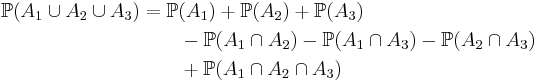
The meaning of the statement is that the number of elements in the union of the two sets is the sum of the elements in each set, respectively, minus the number of elements that are in both. Similarly, for three sets A, B and C,

This can be seen by counting how many times each region in the figure to the right is included in the right hand side.
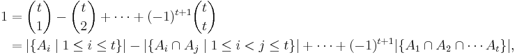
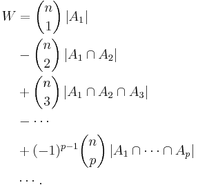
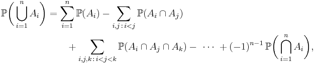
More generally, for finite sets A1, ..., An, one has the identity
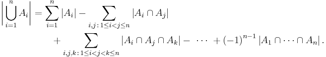
The name comes from the idea that the principle is based on over-generous inclusion, followed by compensating exclusion. When n > 2 the exclusion of the pairwise intersections is (possibly) too severe, and the correct formula is as shown with alternating signs.
This formula is attributed to Abraham de Moivre; it is sometimes also named for Daniel da Silva, Joseph Sylvester or Henri Poincaré.
For the case of three sets A, B, C the inclusion–exclusion principle is illustrated in the graphic on the right.
Contents |
Proof
Let A denote the union  of the sets A1, ..., An. To prove the inclusion–exclusion principle in general, we first have to verify the identity
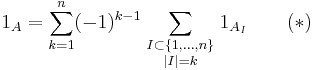
for indicator functions, where
There are at least two ways to do this:
First possibility: It suffices to do this for every x in the union of A1, ..., An. Suppose x belongs to exactly m sets with 1 ≤ m ≤ n, for simplicity of notation say A1, ..., Am. Then the identity at x reduces to
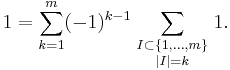
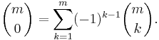
The number of subsets of cardinality k of an m-element set is the combinatorical interpretation of the binomial coefficient  . Since
  , we have
Putting all terms to the left-hand side of the equation, we obtain the expansion for (1 – 1)m given by the binomial theorem, hence we see that (*) is true for x.
Second possibility: The following function is identically zero

because: if x is not in A, then all factors are 0 - 0 = 0; and otherwise, if x does belong to some Am, then the corresponding mth factor is 1 − 1 = 0. By expanding the product on the right-hand side, equation (*) follows.
Use of (*): To prove the inclusion–exclusion principle for the cardinality of sets, sum the equation (*) over all x in the union of A1, ..., An. To derive the version used in probability, take the expectation in (*). In general, integrate the equation (*) with respect to μ. Always use linearity.
Alternative proof
Pick an element contained in the union of all sets and let  be the individual sets containing it. (Note that
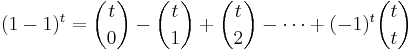
  .) Since the element is counted precisely once by the left-hand side of the equation, we need to show that it is counted only once by the right-hand side. By the binomial theorem,
 .
.
Using the convention that  and rearranging terms, we have
and so the chosen element is indeed counted only once by the right-hand side of the proposed equation.
Example
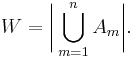
Suppose there is a deck of n cards, each card is numbered from 1 to n. Suppose a card numbered m is in the correct position if it is the mth card in the deck. How many ways, W, can the cards be shuffled with at least 1 card being in the correct position?
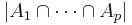
Begin by defining set Am, which is all of the orderings of cards with the mth card correct. Then the number of orders, W, with at least one card being in the correct position, m, is
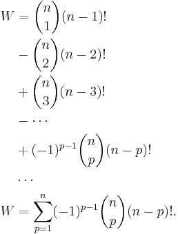
Apply the principle of inclusion-exclusion,
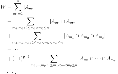
Each value 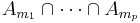 represents the set of shuffles having p values m1, ..., mp in the correct position. Note that the number of shuffles with p values correct only depends on p, not on the particular values of
  . For example, the number of shuffles having the 1st, 3rd, and 17th cards in the correct position is the same as the number of shuffles having the 2nd, 5th, and 13th cards in the correct positions. It only matters that of the n cards, 3 were chosen to be in the correct position. Thus there are
  terms in each summation (see combination).
 is the number of orderings having p elements in the correct position, which is equal to the number of ways of ordering the remaining n − p elements, or (n − p)!. Thus we finally get:
Noting that 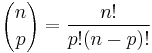 , this reduces to
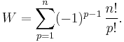
A permutation where no card is in the correct position is called a derangement. Taking n! to be the total number of permutations, the probability Q that a random shuffle produces a derangement is given by
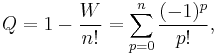
the Taylor expansion of e−1. Thus the probability of guessing an order for a shuffled deck of cards and being incorrect about every card is approximately 1/e or 37%.
In probability
In probability, for events A1, ..., An in a probability space  , the inclusion–exclusion principle becomes for n = 2

for n = 3
and in general
which can be written in closed form as
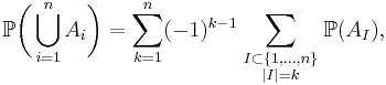
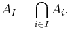
where the last sum runs over all subsets I of the indices 1, ..., n which contain exactly k elements, and
denotes the intersection of all those Ai with index in I.
According to the Bonferroni inequalities, the sum of the first terms in the formula is alternately an upper bound and a lower bound for the LHS. This can be used in cases where the full formula is too cumbersome.
For a general measure space (S,Σ,μ) and measurable subsets A1, ..., An of finite measure, the above identities also hold when the probability measure  is replaced by the measure μ.
Special case
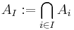
If, in the probabilistic version of the inclusion–exclusion principle, the probability of the intersection AI only depends on the cardinality of I, meaning that for every k in {1, ..., n} there is an ak such that

then the above formula simplifies to
due to the combinatorial interpretation of the binomial coefficient  .
.
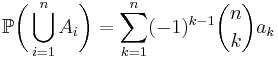
Similarly, when the cardinality of the union of finite sets A1, ..., An is of interest, and these sets are a family with regular intersections, meaning that for every k in {1, ..., n} the intersection
has the same cardinality, say ak = |AI|, irrespective of the k-element subset I of {1, ..., n}, then
An analogous simplification is possible in the case of a general measure space (S,Σ,μ) and measurable subsets A1, ..., An of finite measure.
Diluted inclusion–exclusion principle
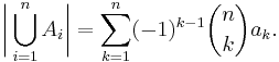
Let A1, ..., An be arbitrary sets and p1, ..., pn real numbers in the closed unit interval [0,1]. Then, for every even number k in {0, ..., n}, the indicator functions satisfy the inequality:[1]
Other forms
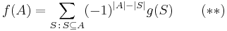
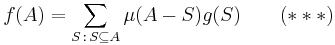
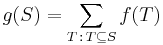
The principle is sometimes stated in the form that says that if
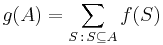
then
-
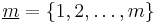
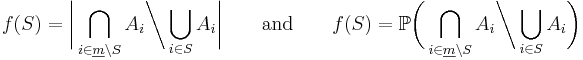
- We show now that the combinatorial and the probabilistic version of the inclusion-exclusion principle are instances of (**). Take
 ,
,  , and
, and
- We show now that the combinatorial and the probabilistic version of the inclusion-exclusion principle are instances of (**). Take
-
- respectively for all sets
 with
with  . Then we obtain
- respectively for all sets

-
- respectively for all sets
 with
with  . This is because elements
  of
of  can be contained in other
  's ('s with
  ) as well, and the
  formula runs exactly through all possible extensions of the sets
 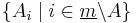 with other 's, counting only for the set that matches the membership behavior of , if runs through all subsets of (as in the definition of
  ).
).
- respectively for all sets
-
- Since , we obtain from (**) with
 that
that
- Since

-
- and by interchanging sides, the combinatorial and the probabilistic version of the inclusion-exclusion principle follow.
If one sees a number  as a set of its prime factors, then (**) is a generalization of Möbius inversion formula for square-free natural numbers. Therefore, (**) is seen as the Möbius inversion formula for the incidence algebra of the partially ordered set of all subsets of A.
For a generalization of the full version of Möbius inversion formula, (**) must be generalized to multisets. For multisets instead of sets, (**) becomes
where  is the multiset for which
 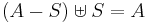 , and
, and
- μ(S) = 1 if S is a set (i.e. a multiset without double elements) of even cardinality.
- μ(S) = −1 if S is a set (i.e. a multiset without double elements) of odd cardinality.
- μ(S) = 0 if S is a proper multiset (i.e. S has double elements).
Notice that 
 is just the
  of (**) in case is a set.
Proof of (***): Substitute
on the right hand side of (***). Notice that  appears once on both sides of (***). So we must show that for all
  with
with  , the terms
  cancel out on the right hand side of (***). For that purpose, take a fixed such that and take an arbitrary fixed
  such that
  .
.
Notice that must be a set for each positive or negative appearance of on the right hand side of (***) that is obtained by way of the multiset such that 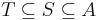 . Now each appearance of on the right hand side of (***) that is obtained by way of such that is a set that contains cancels out with the one that is obtained by way of the corresponding such that is a set that does not contain . This gives the desired result.
Applications
In many cases where the principle could give an exact formula (in particular, counting prime numbers using the sieve of Eratosthenes), the formula arising doesn't offer useful content because the number of terms in it is excessive. If each term individually can be estimated accurately, the accumulation of errors may imply that the inclusion–exclusion formula isn't directly applicable. In number theory, this difficulty was addressed by Viggo Brun. After a slow start, his ideas were taken up by others, and a large variety of sieve methods developed. These for example may try to find upper bounds for the "sieved" sets, rather than an exact formula.
Counting derangements
A well-known application of the inclusion–exclusion principle is to the combinatorial problem of counting all derangements of a finite set. A derangement of a set A is a bijection from A into itself that has no fixed points. Via the inclusion–exclusion principle one can show that if the cardinality of A is n, then the number of derangements is [n! / e] where [x] denotes the nearest integer to x; a detailed proof is available here.
This is also known as the subfactorial of n, written !n. It follows that if all bijections are assigned the same probability then the probability that a random bijection is a derangement quickly approaches 1/e as n grows.
Counting intersections
The principle of inclusion–exclusion, combined with de Morgan's theorem, can be used to count the intersection of sets as well. Let  represent the complement of Ak with respect to some universal set A such that
  for each k. Then we have
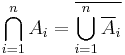
thereby turning the problem of finding an intersection into the problem of finding a union.
See also
- Combinatorial principles
- Boole's inequality
- Necklace problem
- Schuette–Nesbitt formula
- Maximum-minimums identity
Citations
- ^ (Fernández, Fröhlich & Sokal 1992, Proposition 12.6)
References
- Fernández, Roberto; Fröhlich, Jürg; Alan D., Sokal (1992), Random Walks, Critical Phenomena, and Triviality in Quantum Field Theory, Texts an Monographs in Physics, Berlin: Springer-Verlag, pp. xviii+444, ISBN 3-540-54358-9, MR1219313, Zbl 0761.60061
This article incorporates material from principle of inclusion-exclusion on PlanetMath, which is licensed under the Creative Commons Attribution/Share-Alike License.