Condition number
In the field of numerical analysis, the condition number of a function with respect to an argument measures the asymptotically worst case of how much the function can change in proportion to small changes in the argument. The "function" is the solution of a problem and the "arguments" are the data in the problem.
A problem with a low condition number is said to be well-conditioned, while a problem with a high condition number is said to be ill-conditioned.
The condition number is a property of the problem. Paired with the problem are any number of algorithms that can be used to solve the problem, that is, to calculate the solution. Some algorithms have a property called backward stability. In general, a backward stable algorithm can be expected to accurately solve well-conditioned problems. Numerical analysis textbooks give formulas for the condition numbers of problems and identify the backward stable algorithms.
As a general rule of thumb, if the condition number  , then you may lose up to
  digits of accuracy on top of what would be lost to the numerical method due to loss of precision from arithmetic methods.[1] However, the condition number does not give the exact value of the maximum inaccuracy that may occur in the algorithm. It generally just bounds it with an estimate (whose computed value depends on the choice of the norm to measure the inaccuracy).
Contents |
Matrices
For example, the condition number associated with the linear equation Ax = b gives a bound on how inaccurate the solution x will be after approximate solution. Note that this is before the effects of round-off error are taken into account; conditioning is a property of the matrix, not the algorithm or floating point accuracy of the computer used to solve the corresponding system. In particular, one should think of the condition number as being (very roughly) the rate at which the solution, x, will change with respect to a change in b. Thus, if the condition number is large, even a small error in b may cause a large error in x. On the other hand, if the condition number is small then the error in x will not be much bigger than the error in b.
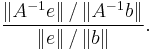
The condition number is defined more precisely to be the maximum ratio of the relative error in x divided by the relative error in b.
Let e be the error in b. Assuming that A is a square matrix, the error in the solution A−1b is A−1e. The ratio of the relative error in the solution to the relative error in b is
This is easily transformed to
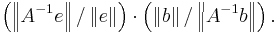
The maximum value (for nonzero b and e) is easily seen to be the product of the two operator norms:
The same definition is used for any consistent norm, i.e. one that satisfies

When the condition number is exactly one, then the algorithm may find an approximation of the solution with an arbitrary precision. However it does not mean that the algorithm will converge rapidly to this solution, just that it won't diverge arbitrarily because of inaccuracy on the source data (backward error), provided that the forward error introduced by the algorithm does not diverge as well because of accumulating intermediate rounding errors.
The condition number may also be infinite, in which case the algorithm will not reliably find a solution to the problem, not even a weak approximation of it (and not even its order of magnitude) with any reasonable and provable accuracy.
Of course, this definition depends on the choice of norm:
- If
 is the norm (usually noted as
  ) defined in the square-summable sequence space ℓ2 (which also matches the usual distance in a continuous and isotropic cartesian space), then
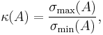
- where
 and
and  are maximal and minimal singular values of
  respectively.
 - Hence
- If is normal then
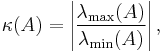
- where
 and
and  are maximal and minimal (by moduli) eigenvalues of respectively.
- If is unitary then
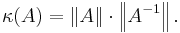
- If
- This number arises so often in numerical linear algebra that it is given a name, the condition number of a matrix.
- If is the norm (usually noted as
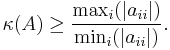
 ) defined in the sequence space ℓ∞ of all bounded sequences (which also matches the non-linear distance measured as the maximum of distances measured on projections into the base subspaces, without requiring the space to be isotropic or even just linear, but only continuous, such norm being definable on all Banach spaces), and is lower triangular non-singular (i.e.,
  ) then
- The condition number computed with this norm is generally larger than the condition number computed with square-summable sequences, but it can be evaluated more easily (and this is often the only measurable condition number, when the problem to solve involves a non-linear algebra, for example when approximating irrational and transcendental functions or numbers with numerical methods.)

Other contexts
Condition numbers can be defined for any function ƒ mapping its data from some domain (e.g. an m-tuple of real numbers x) into some codomain [e.g. an n-tuple of real numbers ƒ(x)], where both the domain and codomain are Banach spaces. They express how sensitive that function is to small changes (or small errors) in its arguments. This is crucial in assessing the sensitivity and potential accuracy difficulties of numerous computational problems, for example polynomial root finding or computing eigenvalues.
The condition number of ƒ at a point x (specifically, its relative condition number[2]) is then defined to be the maximum ratio of the fractional change in ƒ(x) to any fractional change in x, in the limit where the change δx in x becomes infinitesimally small:[2]
![\lim_{ \varepsilon \to 0^%2B }
\sup_{ \Vert \delta x \Vert \leq \varepsilon }
\left[ \frac{ \left\Vert f(x %2B \delta x) - f(x)\right\Vert }{ \Vert f(x) \Vert }
/ \frac{ \Vert \delta x \Vert }{ \Vert x \Vert }
\right],](/2012-wikipedia_en_all_nopic_01_2012/I/fbe98d08a1671533b857bacb2091cd90.png)
where  is a norm on the domain/codomain of ƒ(x).
If ƒ is differentiable, this is equivalent to:[2]
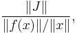
where J denotes the Jacobian matrix of partial derivatives of ƒ and  is the induced norm on the matrix.
References
- ^ Numerical Mathematics and Computing, by Cheney and Kincaid.
- ^ a b c L. N. Trefethen and D. Bau, Numerical Linear Algebra (SIAM, 1997).
External links
- Condition Number of a Matrix at Holistic Numerical Methods Institute
- Matrix condition number on PlanetMath
- MATLAB library function to determine condition number