G-test

In statistics, G-tests are likelihood-ratio or maximum likelihood statistical significance tests that are increasingly being used in situations where chi-squared tests were previously recommended.

The commonly used chi-squared tests for goodness of fit to a distribution and for independence in contingency tables are in fact approximations of the log-likelihood ratio on which the G-tests are based. This approximation was developed by Karl Pearson because at the time it was unduly laborious to calculate log-likelihood ratios. With the advent of electronic calculators and personal computers, this is no longer a problem. G-tests are coming into increasing use, particularly since they were recommended at least since the 1981 edition of the popular statistics textbook by Sokal and Rohlf.^[1] Dunning^[2] introduced the test to the computational linguistics community where it is now widely used.

The general formula for Pearson's chi-squared test statistic is

$\Chi^2 = \sum_{ij} {(O_{ij} - E_{ij})^2 \over E_{ij}} ,$

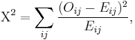
where O_i is the frequency observed in a cell, E is the frequency expected on the null hypothesis, and the sum is taken across all cells. The corresponding general formula for G is

$G = 2\sum_{ij} {O_{ij} \cdot \ln(O_{ij}/E_{ij}) },$

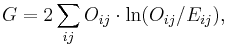
where ln denotes the natural logarithm (log to the base e) and the sum is again taken over all non-empty cells.

1 Relation to mutual information
2 Distribution and usage
3 Application
4 Statistical software
5 References

Relation to mutual information

The value of G can also be expressed in terms of mutual information.

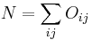
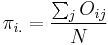
Let

$N = \sum_{ij}{O_{ij}} \,$ , $\pi_{ij} = {O_{ij} \over N}$ , $\pi_{i.} = {\sum_j O_{ij} \over N}$ and $\pi_{. j} = {\sum_i O_{ij} \over N} .$

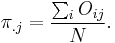
Then G can be expressed in several alternative forms:

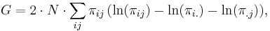
$G = 2 \cdot N \cdot \sum_{ij}{\pi_{ij} \left( \ln(\pi_{ij})-\ln(\pi_{i.})-\ln(\pi_{.j}) \right)} ,$

$G = 2 \cdot N \cdot \left[ H(row) %2B H(col) - H(row,col) \right] ,$

$G = 2 \cdot N \cdot MI(row,col) \, ,$

where the entropy of a discrete random variable $X \,$ is defined as

$H(X) = - {\sum_x p(x) log p(x)} \, ,$

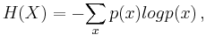
and where

$MI(row,col)= H(row) %2B H(col) - H(row,col) \,$

is the mutual information between the row vector and the column vector of the contingency table.

It can also be shown that the inverse document frequency weighting commonly used for text retrieval is an approximation of G applicable when the row sum for the query is much smaller than the row sum for the remainder of the corpus. Similarly, the result of Bayesian inference applied to a choice of single multinomial distribution for all rows of the contingency table taken together versus the more general alternative of a separate multinomial per row produces results very similar to the G statistic.

Distribution and usage

Given the null hypothesis that the observed frequencies result from random sampling from a distribution with the given expected frequencies, the distribution of G is approximately a chi-squared distribution, with the same number of degrees of freedom as in the corresponding chi-squared test.

For samples of a reasonable size, the G-test and the chi-squared test will lead to the same conclusions. However, the approximation to the theoretical chi-squared distribution for the G-test is better than for the Pearson chi-squared tests in cases where for any cell 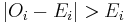$| O_i - E_i | > E_i$ , and in any such case the G-test should always be used.

For very small samples the multinomial test for goodness of fit, and Fisher's exact test for contingency tables, or even Bayesian hypothesis selection are preferable to either the chi-squared test or the G-test.

Application

An application of the G-test is known as the McDonald–Kreitman test in statistical genetics.

Statistical software

Software for the R programming language (homepage here) to perform the G-test is available on a Professor's software page at the University of Alberta.
Fisher's G-Test in the GeneCycle Package of the R programming language (fisher.g.test) does not implement the G-test as described in this article, but rather Fisher's exact test of Gaussian white-noise in a time series (see Fisher, R.A. 1929 "Tests of significance in harmonic analysis").
In SAS, one can conduct G-Test by applying the /chisq option in proc freq.^[3]

References

^ Sokal, R. R. and Rohlf, F. J. (1981). Biometry: the principles and practice of statistics in biological research., New York: Freeman. ISBN 0-7167-2411-1.
^ Dunning, Ted (1993). Accurate Methods for the Statistics of Surprise and Coincidence, Computational Linguistics, Volume 19, issue 1 (March, 1993).
^ G-Test in Handbook of Biological Statistics, University of Delaware.