Frequency-resolved optical gating
In optics, frequency-resolved optical gating (FROG) is a derivative of autocorrelation, but is far superior in its ability to measure ultrafast optical pulse shapes. Further, it can determine the phase of the pulse. In the most common configuration, FROG is simply a background-free autocorrelator followed by a spectrometer. It is the two-dimensional nature of the FROG trace that allows the extraction of the actual pulse shape and phase from the data.
Contents |
The basics
Frequency-Resolved refers to the fact that the final signal is a spectrum. Before explaining Optical Gating, it helps to recognize that the pulse is really interacting with itself. In most configurations, the pulse is split and recombined, as in an interferometer. However, in this case, the recombination does not occur on a beam-splitter, but rather in a nonlinear medium, which allows the two beams to interact with each other. It is this interaction that allows the pulses to "gate" the spectral information of the other pulse. So Optical Gating refers to the fact that the measured spectrum is really from a time-slice of the pulse, and that time-slice is determined by the pulse nonlinear interaction. The gate function depends on the type of nonlinear interaction allowed.
Mathematically the FROG trace is simply a spectrogram but with an unknown gate function:
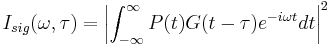
where  is the "probe" pulse and
  is the "gate" pulse. The probe and gate pulses are determined by the nonlinear interaction used, and it is the form of the probe and gate that distinguishes the different types of FROG from each other. Some of the most common are:
 |
 |
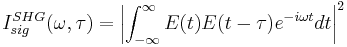
: Second-harmonic generation FROG |
 |
 |
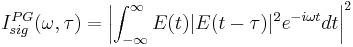
: Polarization gating FROG |
 |
 |
: Self-diffraction FROG |
 |
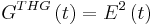 |
: Third-harmonic generation FROG |
For example second-harmonic generation FROG (SHG FROG) would be:
and PG FROG would be:
Traditional inversion algorithms for spectrograms requires perfect knowledge of the gate function (), however, FROG does not have this luxury. Instead an iterative alogrithm is used. The algorithm uses both the data (FROG trace) and form of the nonlinearity to achieve a best match between the real FROG trace and the "retrieved" FROG trace. The retrieved FROG trace is created synthetically from the best guess for  .
.
FROG algorithm
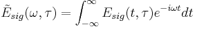
The FROG algorithm is all about phase retrieval. The FROG trace measured in the lab is the exact intensity of  ; however, it is missing the phase information. To start off with define a signal field:
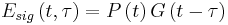
and further defining:
given this the FROG trace becomes:
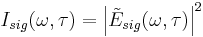
inverting this:
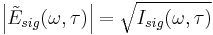
so the amplitude of  is known, but not its phase. If this phase is found, then the pulse () can be retrieved.
An iterative algorithm is used to determine this unknown phase.
- Start with an initial guess for
 .
. - Synthetically create
 from .
 - Fourier transform the time axis to the frequency domain, yielding .
- Compare
 to
to  (generally the rms difference). If this error (termed the "G" error) is sufficiently small, exit the loop.
 - Replace the amplitude (preserving the phase) of with the amplitude measured in the lab (). Call this
 .
. - Take and inverse Fourier transform it back into the time domain (
 ).
). - Extract the best from .
- GOTO 2.
See also
FROG techniques
- Grating-eliminated no-nonsense observation of ultrafast incident laser light e-fields (GRENOUILLE), a simplified version of FROG
Competing techniques
- Spectral phase interferometry for direct electric-field reconstruction (SPIDER)
- Streak camera — not a significant competitor. Streak cameras have picosecond response times.
- Multiphoton intrapulse interference phase scan (MIIPS), a method to characterize and manipulate the ultrashort pulse.
- Frequency-resolved electro-absorption gating (FREAG)
References
- Rick Trebino (2002). Frequency-Resolved Optical Gating: The Measurement of Ultrashort Laser Pulses. Springer. ISBN 1-4020-7066-7.
Controversy
In their 2007 paper, "Amplitude ambiguities in second-harmonic generation frequency-resolved optical gating", B. Yellampalle, K. Y. Kim, and A. J. Taylor, in Optics Letters, Vol. 32, Issue 24, pp. 3558–3560. Yellampalle et al. raised concerns (shown later to be in error) about FROG. Trebino found a calculation error that was a fatal flaw in their paper, and sought to have his clarification published as a comment in the journal. However, Trebino had some challenges in getting his response to the paper published as a comment, a saga he relates with much endurance and some humor in "How to Publish a Scientific Comment in 123 Easy Steps" [1]
A reply to L. Xu, D. J. Kane, and R. Trebino, "Amplitude ambiguities in second-harmonic-generation frequency-resolved optical gating: comment," Opt. Lett. 34, 2602-2602 (2009) is given in B. Yellampalle, K. Kim, and A. J. Taylor, "Amplitude ambiguities in second-harmonic-generation frequency-resolved optical gating: reply to comment," Opt. Lett. 34, 2603-2603 (2009). In their reply Yellampalle et al. insist in their concern and remind the readership that the "FROG algorithms do not produce correct results nearly 20% of the time for complex or multiple pulses."
Also, researchers are actively working on simpler more direct methods to determine the pulse shape of femtosecond and attosecond lasers, see for example the work of J. Gagnon and V. S. Yakolev, Appl. Phys. B 103, 303-309 (2011).
External links
- FROG Page by Rick Trebino (co-inventor of FROG)