Exponential growth
Exponential growth (including exponential decay when the growth rate is negative) occurs when the growth rate of the value of a mathematical function is proportional to the function's current value. In the case of a discrete domain of definition with equal intervals it is also called geometric growth or geometric decay (the function values form a geometric progression).
The formula for exponential growth of a variable x at the (positive or negative) growth rate r, as time t goes on in discrete intervals (that is, at integer times 0, 1, 2, 3, ...), is
where  is the value of x at time 0. For example, with a growth rate of r = 5% = 0.05, going from any integer value of time to the next integer causes x at the second time to be 1.05 times (i.e., 5% larger than) what it was at the previous time.
The exponential growth model is also known as the Malthusian growth model. US scholar Albert Bartlett pointed out the difficulty to grasp ramifications of exponential growth, stating: "The greatest shortcoming of the human race is our inability to understand the exponential function."[1]
Contents |
Examples
- Biology
- The number of microorganisms in a culture both will grow exponentially until an essential nutrient is exhausted. Typically the first organism splits into two daughter organisms, who then each split to form four, who split to form eight, and so on.
- A virus (for example SARS, or smallpox) typically will spread exponentially at first, if no artificial immunization is available. Each infected person can infect multiple new people.
- Human population, if the number of births and deaths per person per year were to remain at current levels (but also see logistic growth). For example, according to the United States Census Bureau, over the last 100 years (1910 to 2010), the population of the United States of America is exponentially increasing at an average rate of one and a half percent a year (1.5%). This means that the doubling time of the American population (depending on the yearly growth in population) is approximately 50 years.[2]
- Many responses of living beings to stimuli, including human perception, are logarithmic responses, which are the inverse of exponential responses; the loudness and frequency of sound are perceived logarithmically, even with very faint stimulus, within the limits of perception. This is the reason that exponentially increasing the brightness of visual stimuli is perceived by humans as a linear increase, rather than an exponential increase. This has survival value. Generally it is important for the organisms to respond to stimuli in a wide range of levels, from very low levels, to very high levels, while the accuracy of the estimation of differences at high levels of stimulus is much less important for survival.
- Physics
- Avalanche breakdown within a dielectric material. A free electron becomes sufficiently accelerated by an externally applied electrical field that it frees up additional electrons as it collides with atoms or molecules of the dielectric media. These secondary electrons also are accelerated, creating larger numbers of free electrons. The resulting exponential growth of electrons and ions may rapidly lead to complete dielectric breakdown of the material.
- Nuclear chain reaction (the concept behind nuclear reactors and nuclear weapons). Each uranium nucleus that undergoes fission produces multiple neutrons, each of which can be absorbed by adjacent uranium atoms, causing them to fission in turn. If the probability of neutron absorption exceeds the probability of neutron escape (a function of the shape and mass of the uranium), k > 0 and so the production rate of neutrons and induced uranium fissions increases exponentially, in an uncontrolled reaction. "Due to the exponential rate of increase, at any point in the chain reaction 99% of the energy will have been released in the last 4.6 generations. It is a reasonable approximation to think of the first 53 generations as a latency period leading up to the actual explosion, which only takes 3–4 generations."[3]
- Positive feedback within the linear range of electrical or electroacoustic amplification can result in the exponential growth of the amplified signal, although resonance effects may favor some component frequencies of the signal over others.
- Heat transfer experiments yield results whose best fit line are exponential decay curves.
- Economics
- Economic growth is expressed in percentage terms, implying exponential growth. For example, U.S. GDP per capita has grown at an exponential rate of approximately two percent per year for two centuries.
- Multi-level marketing. Exponential increases are promised to appear in each new level of a starting member's downline as each subsequent member recruits more people.
- Finance
- Compound interest at a constant interest rate provides exponential growth of the capital. See also rule of 72.
- Pyramid schemes or Ponzi schemes also show this type of growth resulting in high profits for a few initial investors and losses among great numbers of investors.
- Computer technology
- Processing power of computers. See also Moore's law and technological singularity (under exponential growth, there are no singularities. The singularity here is a metaphor.).
- In computational complexity theory, computer algorithms of exponential complexity require an exponentially increasing amount of resources (e.g. time, computer memory) for only a constant increase in problem size. So for an algorithm of time complexity 2x, if a problem of size x = 10 requires 10 seconds to complete, and a problem of size x = 11 requires 20 seconds, then a problem of size x = 12 will require 40 seconds. This kind of algorithm typically becomes unusable at very small problem sizes, often between 30 and 100 items (most computer algorithms need to be able to solve much larger problems, up to tens of thousands or even millions of items in reasonable times, something that would be physically impossible with an exponential algorithm). Also, the effects of Moore's Law do not help the situation much because doubling processor speed merely allows you to increase the problem size by a constant. E.g. if a slow processor can solve problems of size x in time t, then a processor twice as fast could only solve problems of size x+constant in the same time t. So exponentially complex algorithms are most often impractical, and the search for more efficient algorithms is one of the central goals of computer science today.
- Internet traffic growth.
Basic formula
A quantity x depends exponentially on time t if
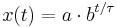
where the constant a is the initial value of x,

and the constant b is a positive growth factor, and τ is the time required for x to increase by a factor of b:
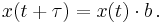
If τ > 0 and b > 1, then x has exponential growth. If τ < 0 and b > 1, or τ > 0 and 0 < b < 1, then x has exponential decay.
Example: If a species of bacteria doubles every ten minutes, starting out with only one bacterium, how many bacteria would be present after one hour? The question implies a = 1, b = 2 and τ = 10 min.

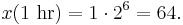
After one hour, or six ten-minute intervals, there would be sixty-four bacteria.
Many pairs (b, τ) of a dimensionless non-negative number b and an amount of time τ (a physical quantity which can be expressed as the product of a number of units and a unit of time) represent the same growth rate, with τ proportional to log b. For any fixed b not equal to 1 (e.g. e or 2), the growth rate is given by the non-zero time τ. For any non-zero time τ the growth rate is given by the dimensionless positive number b.
Thus the law of exponential growth can be written in different but mathematically equivalent forms, by using a different base. The most common forms are the following:

where x0 expresses the initial quantity x(0).
Parameters (negative in the case of exponential decay):
- The growth constant k is the frequency (number of times per unit time) of growing by a factor e; in finance it is also called the logarithmic return, continuously compounded return, or force of interest.
- The e-folding time
 is the time it takes to grow by a factor e.
 - The doubling time T is the time it takes to double.
- The percent increase r (a dimensionless number) in a period p.
The quantities k, , and T, and for a given p also r, have a one-to-one connection given by the following equation (which can be derived by taking the natural logarithm of the above):
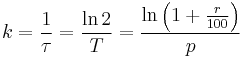
where k = 0 corresponds to r = 0 and to and T being infinite.
If p is the unit of time the quotient t/p is simply the number of units of time. Using the notation t for the (dimensionless) number of units of time rather than the time itself, t/p can be replaced by t, but for uniformity this has been avoided here. In this case the division by p in the last formula is not a numerical division either, but converts a dimensionless number to the correct quantity including unit.
A popular approximated method for calculating the doubling time from the growth rate is the rule of 70, i.e.  .
.
Reformulation as log-linear growth
If a variable x exhibits exponential growth according to 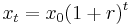 , then the log (to any base) of x grows linearly over time, as can be seen by taking logarithms of both sides of the exponential growth equation:

This allows an exponentially growing variable to be modeled with a log-linear model. For example, if one wishes to empirically estimate the growth rate from intertemporal data on x, one can linearly regress log x on t.
Differential equation
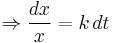
The exponential function  satisfies the linear differential equation:

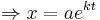
saying that the growth rate of x at time t is proportional to the value of x(t), and it has the initial value

For  the differential equation is solved by the method of separation of variables:

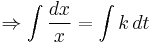

Incorporating the initial value gives:
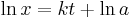
The solution also applies for  where the logarithm is not defined.
For a nonlinear variation of this growth model see logistic function.
Difference equation
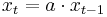
has solution
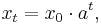
showing that x experiences exponential growth.
Other growth rates
In the long run, exponential growth of any kind will overtake linear growth of any kind (the basis of the Malthusian catastrophe) as well as any polynomial growth, i.e., for all α:
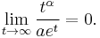
There is a whole hierarchy of conceivable growth rates that are slower than exponential and faster than linear (in the long run). See Degree of a polynomial#The degree computed from the function values.
Growth rates may also be faster than exponential.
In the above differential equation, if k < 0, then the quantity experiences exponential decay.
Limitations of models
Exponential growth models of physical phenomena only apply within limited regions, as unbounded growth is not physically realistic. Although growth may initially be exponential, the modelled phenomena will eventually enter a region in which previously ignored negative feedback factors become significant (leading to a logistic growth model) or other underlying assumptions of the exponential growth model, such as continuity or instantaneous feedback, break down.
Exponential stories
Rice on a chessboard
According to legend, vizier Sissa Ben Dahir presented an Indian King Sharim with a beautiful, hand-made chessboard. The king asked what he would like in return for his gift and the courtier surprised the king by asking for one grain of rice on the first square, two grains on the second, four grains on the third etc. The king readily agreed and asked for the rice to be brought. All went well at first, but the requirement for 2 n − 1 grains on the nth square demanded over a million grains on the 21st square, more than a million million (aka trillion) on the 41st and there simply was not enough rice in the whole world for the final squares. (from Swirski, 2006)
For variation of this see second half of the chessboard in reference to the point where an exponentially growing factor begins to have a significant economic impact on an organization's overall business strategy.
The water lily
French children are told a story in which they imagine having a pond with water lily leaves floating on the surface. The lily population doubles in size every day and if left unchecked will smother the pond in 30 days, killing all the other living things in the water. Day after day the plant seems small and so it is decided to leave it to grow until it half-covers the pond, before cutting it back. They are then asked, on what day that will occur. This is revealed to be the 29th day, and then there will be just one day to save the pond. (From Meadows et al. 1972, p. 29 via Porritt 2005)
See also
References
- ^ Bartlett, Albert (2004). The Essential Exponential! For the Future of Our Planet. Center for Science, Mathematics and Computer Education, University of Nebraska-Lincoln. ISBN 0-9758973-0-6. http://scimath.unl.edu/exp/expmain.html. Retrieved 2011-06-15. See also the author's video lecture: Arithmetic, Population and Energy.
- ^ 2010 Census Data. “U.S. Census Bureau.” 12 Nov. 2011. http://2010.census.gov/2010census/data/index.php
- ^ Sublette, Carey. "Introduction to Nuclear Weapon Physics and Design". Nuclear Weapons Archive. http://nuclearweaponarchive.org/Nwfaq/Nfaq2.html. Retrieved 2009-05-26.
Sources
- Meadows, Donella H., Dennis L. Meadows, Jørgen Randers, and William W. Behrens III. (1972) The Limits to Growth. New York: University Books. ISBN 0-87663-165-0
- Porritt, J. Capitalism as if the world matters, Earthscan 2005. ISBN 1-84407-192-8
- Swirski, Peter. Of Literature and Knowledge: Explorations in Narrative Thought Experiments, Evolution, and Game Theory. New York: Routledge. ISBN: 0415420601
- Thomson, David G. Blueprint to a Billion: 7 Essentials to Achieve Exponential Growth, Wiley Dec 2005, ISBN 0-471-74747-5
- Tsirel, S. V. 2004. On the Possible Reasons for the Hyperexponential Growth of the Earth Population. Mathematical Modeling of Social and Economic Dynamics / Ed. by M. G. Dmitriev and A. P. Petrov, pp. 367–9. Moscow: Russian State Social University, 2004.
External links
- Exponent calculator — One of the best ways to see how exponents work is to simply try different examples. This calculator enables you to enter an exponent and a base number and see the result.
- Exponential Growth Calculator — This calculator enables you to perform a variety of calculations relating to exponential consumption growth.
- Understanding Exponential Growth — video clip 8.5 min
- Growth in a Finite World - Sustainability and the Exponential Function — Presentation
- Dr. Albert Bartlett: Arithmetic, Population and Energy — streaming video and audio 58 min