Electrical resistivity and conductivity

Electrical resistivity (also known as resistivity, specific electrical resistance, or volume resistivity) is a measure of how strongly a material opposes the flow of electric current. A low resistivity indicates a material that readily allows the movement of electric charge. The SI unit of electrical resistivity is the ohm metre (Ωm). It is commonly represented by the Greek letter ρ (rho).

Electrical conductivity or specific conductance is the reciprocal quantity, and measures a material's ability to conduct an electric current. It is commonly represented by the Greek letter σ (sigma), but κ (esp. in electrical engineering) or γ are also occasionally used. Its SI unit is siemens per metre (S·m⁻¹) and CGSE unit is reciprocal second (s⁻¹):

Contents 1 Definitions 1.1 Scalar form 1.2 Tensor generalization 2 Causes of resistivity 2.1 Band theory simplified 2.2 In metals 2.3 In semiconductors and insulators 2.4 In ionic liquids/electrolytes 3 Resistivity of various materials 4 Temperature dependence 4.1 Linear approximation 4.2 Metals 4.3 Semiconductors 5 Complex resistivity and conductivity 6 Resistivity density products 7 See also 8 Notes and references 9 Further reading 10 External links

Definitions

Scalar form

Electrical resistivity ρ (Greek: rho) is defined by,

where

ρ is the static resistivity (measured in ohm-metres, Ω-m)

E is the magnitude of the electric field (measured in volts per metre, V/m),

J is the magnitude of the current density (measured in amperes per square metre, A/m²),

and E and J are both inside the conductor.

Many resistors and conductors have a uniform cross section with a uniform flow of electric current and are made of one material. (See the diagram to the right.) In this case, the above definition of ρ leads to:

where

R is the electrical resistance of a uniform specimen of the material (measured in ohms, Ω)

is the length of the piece of material (measured in metres, m)

A is the cross-sectional area of the specimen (measured in square metres, m²).

The reason resistivity has the dimension units of ohm-metres can be seen by transposing the definition to make resistance the subject:

The resistance of a given sample will increase with the length, but decrease with greater cross-sectional area. Resistance is measured in ohms. Length over area has units of 1/distance. To end up with ohms, resistivity must be in the units of "ohms×distance" (SI ohm-metre, US ohm-inch).

In a hydraulic analogy, increasing the cross-sectional area of a pipe reduces its resistance to flow, and increasing the length increases resistance to flow (and pressure drop for a given flow).

Tensor generalization

The scalar equation:

or equivalently

is only valid for resistors and conductors which are homogeneous and isotropic, that is the conductivity is uniform throughout the conductor, carrying a uniform electric current per unit cross-sectional area J, through a uniform internal electric field E, all in one dimension only.

For all three dimensions we have at all points (r = position vector at a point in the conductor):

in which (1, 2, 3 refer to components)

This is still only true if E and J are collinear, under the same conditions as above.

Since E and J are generally vector fields, the material may not be homogeneous or isotropic so the conductivity may vary from point to point, and the E and J are not always collinear at the same point, the definition generalizes by treating conductivity as a rank-2 tensor field σ:

where rank-2 tensors can be represented by matrices

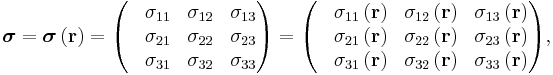
equivalent to the matrix equation

which allows a simple relation between components to be read off, using the Einstein summation convention;

^[1]

The above tensor equation serves as a definition for the conductivity tensor (or field). A similar analysis for resistivity can be done, introducing a resistivity tensor (or field) in an identical form,

in which

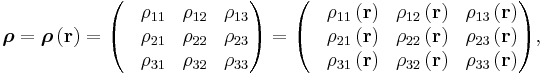
so

Causes of resistivity

Band theory simplified

Quantum mechanics states that the energy of an electron in an atom cannot be any arbitrary value. Rather, there are fixed energy levels which the electrons can occupy, and values in between these levels are impossible. The energy levels are grouped into two bands: the valence band and the conduction band (the latter is generally above the former). Electrons in the conduction band may move freely throughout the substance in the presence of an electrical field.

In insulators and semiconductors, the atoms in the substance influence each other so that between the valence band and the conduction band there exists a forbidden band of energy levels, which the electrons cannot occupy. In order for a current to flow, a relatively large amount of energy must be furnished to an electron for it to leap across this forbidden gap and into the conduction band. Thus, even large voltages can yield relatively small currents.

In metals

A metal consists of a lattice of atoms, each with a shell of electrons. This is also known as a positive ionic lattice. The outer electrons are free to dissociate from their parent atoms and travel through the lattice, creating a 'sea' of electrons, making the metal a conductor. When an electrical potential difference (a voltage) is applied across the metal, the electrons drift from one end of the conductor to the other under the influence of the electric field.

Near room temperatures, the thermal motion of ions is the primary source of scattering of electrons (due to destructive interference of free electron waves on non-correlating potentials of ions), and is thus the prime cause of metal resistance. Imperfections of lattice also contribute into resistance, although their contribution in pure metals is negligible.

The larger the cross-sectional area of the conductor, the more electrons are available to carry the current, so the lower the resistance. The longer the conductor, the more scattering events occur in each electron's path through the material, so the higher the resistance. Different materials also affect the resistance.^[2]

In semiconductors and insulators

In metals, the Fermi level lies in the conduction band (see Band Theory, below) giving rise to free conduction electrons. However, in semiconductors the position of the Fermi level is within the band gap, approximately half-way between the conduction band minimum and valence band maximum for intrinsic (undoped) semiconductors. This means that at 0 kelvins, there are no free conduction electrons and the resistance is infinite. However, the resistance will continue to decrease as the charge carrier density in the conduction band increases. In extrinsic (doped) semiconductors, dopant atoms increase the majority charge carrier concentration by donating electrons to the conduction band or accepting holes in the valence band. For both types of donor or acceptor atoms, increasing the dopant density leads to a reduction in the resistance. Highly doped semiconductors hence behave metallic. At very high temperatures, the contribution of thermally generated carriers will dominate over the contribution from dopant atoms and the resistance will decrease exponentially with temperature.

In ionic liquids/electrolytes

In electrolytes, electrical conduction happens not by band electrons or holes, but by full atomic species (ions) traveling, each carrying an electrical charge. The resistivity of ionic liquids varies tremendously by the concentration - while distilled water is almost an insulator, salt water is a very efficient electrical conductor. In biological membranes, currents are carried by ionic salts. Small holes in the membranes, called ion channels, are selective to specific ions and determine the membrane resistance.

Resistivity of various materials

• A conductor such as a metal has high conductivity and a low resistivity.
• An insulator like glass has low conductivity and a high resistivity.
• The conductivity of a semiconductor is generally intermediate, but varies widely under different conditions, such as exposure of the material to electric fields or specific frequencies of light, and, most important, with temperature and composition of the semiconductor material.

The degree of doping in semiconductors makes a large difference in conductivity. To a point, more doping leads to higher conductivity. The conductivity of a solution of water is highly dependent on its concentration of dissolved salts, and other chemical species that ionize in the solution. Electrical conductivity of water samples is used as an indicator of how salt-free, ion-free, or impurity-free the sample is; the purer the water, the lower the conductivity (the higher the resistivity). Conductivity measurements in water are often reported as specific conductance, relative to the conductivity of pure water at 25 °C. An EC meter is normally used to measure conductivity in a solution. A rough summary is as follows:

Material	Resistivity ρ (Ω·m)
Metals	10−8
Semiconductors	variable
Electrolytes	variable
Insulators	1016
Superconductors	0

This table shows the resistivity, conductivity and temperature coefficient of various materials at 20 °C (68 °F)

Material	ρ (Ω·m) at 20 °C	σ (S/m) at 20 °C	Temperature coefficient[note 1] (K−1)	Reference
Silver	1.59×10−8	6.30×107	0.0038	[3][4]
Copper	1.68×10−8	5.96×107	0.0039	[4]
Annealed copper[note 2]	1.72×10−8	5.80×107
Gold[note 3]	2.44×10−8	4.10×107	0.0034	[3]
Aluminium[note 4]	2.82×10−8	3.5×107	0.0039	[3]
Calcium	3.36×10−8	2.98×107	0.0041
Tungsten	5.60×10−8	1.79×107	0.0045	[3]
Zinc	5.90×10−8	1.69×107	0.0037	[5]
Nickel	6.99×10−8	1.43×107	0.006
Lithium	9.28×10−8	1.08×107	0.006
Iron	1.0×10−7	1.00×107	0.005	[3]
Platinum	1.06×10−7	9.43×106	0.00392	[3]
Tin	1.09×10−7	9.17×106	0.0045
Lead	2.2×10−7	4.55×106	0.0039	[3]
Titanium	4.20×10−7	2.38×106	X
Manganin	4.82×10−7	2.07×106	0.000002	[6]
Constantan	4.9×10−7	2.04×106	0.000008	[7]
Stainless steel[note 5]	6.9×10−7	1.45×106		[8]
Mercury	9.8×10−7	1.02×106	0.0009	[6]
Nichrome[note 6]	1.10×10−6	9.09×105	0.0004	[3]
Carbon (amorphous)	5×10−4 to 8×10−4	1.25 to 2×103	−0.0005	[3][9]
Carbon (graphite)[note 7]	2.5e×10−6 to 5.0×10−6 ⊥basal plane 3.0×10−3 //basal plane	2 to 3×105 ⊥basal plane 3.3×102 //basal plane		[10]
Carbon (diamond)[note 8]	1×1012	~10−13		[11]
Germanium[note 8]	4.6×10−1	2.17	−0.048	[3][4]
Sea water[note 9]	2×10−1	4.8		[12]
Drinking water[note 10]	2×101 to 2×103	5×10−4 to 5×10−2
Deionized water[note 11]	1.8×105	5.5×10−6		[13]
Silicon[note 8]	6.40×102	1.56×10−3	−0.075	[3]
GaAs	5×10−7 to 10×10−3	5×10−8 to 103		[14]
Glass	10×1010 to 10×1014	10−11 to 10−15	?	[3][4]
Hard rubber	1×1013	10−14	?	[3]
Sulfur	1×1015	10−16	?	[3]
Air	1.3×1016 to 3.3×1016	3 to 8×10−15		[15]
Paraffin	1×1017	10−18	?
Fused quartz	7.5×1017	1.3×10−18	?	[3]
PET	10×1020	10−21	?
Teflon	10×1022 to 10×1024	10−25 to 10−23	?

The effective temperature coefficient varies with temperature and purity level of the material. The 20 °C value is only an approximation when used at other temperatures. For example, the coefficient becomes lower at higher temperatures for copper, and the value 0.00427 is commonly specified at 0 °C.^[16]

The extremely low resistivity (high conductivity) of silver is characteristic of metals. George Gamow tidily summed up the nature of the metals' dealings with electrons in his science-popularizing book, One, Two, Three...Infinity (1947): "The metallic substances differ from all other materials by the fact that the outer shells of their atoms are bound rather loosely, and often let one of their electrons go free. Thus the interior of a metal is filled up with a large number of unattached electrons that travel aimlessly around like a crowd of displaced persons. When a metal wire is subjected to electric force applied on its opposite ends, these free electrons rush in the direction of the force, thus forming what we call an electric current." More technically, the free electron model gives a basic description of electron flow in metals.

Temperature dependence

Linear approximation

The electrical resistivity of most materials changes with temperature. If the temperature T does not vary too much, a linear approximation is typically used:

where is called the temperature coefficient of resistivity, is a fixed reference temperature (usually room temperature), and is the resistivity at temperature . The parameter is an empirical parameter fitted from measurement data. Because the linear approximation is only an approximation, is different for different reference temperatures. For this reason it is usual to specify the temperature that was measured at with a suffix, such as , and the relationship only holds in a range of temperatures around the reference.^[17] When the temperature varies over a large temperature range, the linear approximation is inadequate and a more detailed analysis and understanding should be used.

Metals

In general, electrical resistivity of metals increases with temperature. Electron–phonon interactions can play a key role. At high temperatures, the resistance of a metal increases linearly with temperature. As the temperature of a metal is reduced, the temperature dependence of resistivity follows a power law function of temperature. Mathematically the temperature dependence of the resistivity ρ of a metal is given by the Bloch–Grüneisen formula:

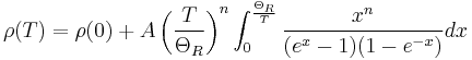
where is the residual resistivity due to defect scattering, A is a constant that depends on the velocity of electrons at the Fermi surface, the Debye radius and the number density of electrons in the metal. is the Debye temperature as obtained from resistivity measurements and matches very closely with the values of Debye temperature obtained from specific heat measurements. n is an integer that depends upon the nature of interaction:

1. n=5 implies that the resistance is due to scattering of electrons by phonons (as it is for simple metals)
2. n=3 implies that the resistance is due to s-d electron scattering (as is the case for transition metals)
3. n=2 implies that the resistance is due to electron–electron interaction.

If more than one source of scattering is simultaneously present, Matthiessen's Rule (first formulated by Augustus Matthiessen in the 1860s) ^[18][19] says that the total resistance can be approximated by adding up several different terms, each with the appropriate value of n.

As the temperature of the metal is sufficiently reduced (so as to 'freeze' all the phonons), the resistivity usually reaches a constant value, known as the residual resistivity. This value depends not only on the type of metal, but on its purity and thermal history. The value of the residual resistivity of a metal is decided by its impurity concentration. Some materials lose all electrical resistivity at sufficiently low temperatures, due to an effect known as superconductivity.

An investigation of the low-temperature resistivity of metals was the motivation to Heike Kamerlingh Onnes's experiments that led in 1911 to discovery of superconductivity. For details see History of superconductivity.

Semiconductors

In general, resistivity of intrinsic semiconductors decreases with increasing temperature. The electrons are bumped to the conduction energy band by thermal energy, where they flow freely and in doing so leave behind holes in the valence band which also flow freely. The electric resistance of a typical intrinsic (non doped) semiconductor decreases exponentially with the temperature:

An even better approximation of the temperature dependence of the resistivity of a semiconductor is given by the Steinhart–Hart equation:

where A, B and C are the so-called Steinhart–Hart coefficients.

This equation is used to calibrate thermistors.

Extrinsic (doped) semiconductors have a far more complicated temperature profile. As temperature increases starting from absolute zero they first decrease steeply in resistance as the carriers leave the donors or acceptors. After most of the donors or acceptors have lost their carriers the resistance starts to increase again slightly due to the reducing mobility of carriers (much as in a metal). At higher temperatures it will behave like intrinsic semiconductors as the carriers from the donors/acceptors become insignificant compared to the thermally generated carriers.^[20]

In non-crystalline semiconductors, conduction can occur by charges quantum tunnelling from one localised site to another. This is known as variable range hopping and has the characteristic form of 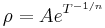, where n=2,3,4 depending on the dimensionality of the system.

Complex resistivity and conductivity

When analyzing the response of materials to alternating electric fields, in applications such as electrical impedance tomography,^[21] it is necessary to replace resistivity with a complex quantity called impeditivity (in analogy to electrical impedance). Impeditivity is the sum of a real component, the resistivity, and an imaginary component, the reactivity (in analogy to reactance). The magnitude of Impeditivity is the square root of sum of squares of magnitudes of resistivity and reactivity.

Conversely, in such cases the conductivity must be expressed as a complex number (or even as a matrix of complex numbers, in the case of anisotropic materials) called the admittivity. Admittivity is the sum of a real component called the conductivity and an imaginary component called the susceptivity.

An alternative description of the response to alternating currents uses a real (but frequency-dependent) conductivity, along with a real permittivity. The larger the conductivity is, the more quickly the alternating-current signal is absorbed by the material (i.e., the more opaque the material is). For details, see Mathematical descriptions of opacity.

Resistivity density products

In some applications where the weight of an item is very important resistivity density products are more important than absolute low resistivity- it is often possible to make the conductor thicker to make up for a higher resistivity; and then a low resistivity density product material (or equivalently a high conductance to density ratio) is desirable. For example, for long distance overhead power lines— aluminium is frequently used rather than copper because it is lighter for the same conductance.

Material	Resistivity (nΩ·m)	Density (g/cm3)	Resistivity-density product (nΩ·m·g/cm3)
Sodium	47.7	0.97	46
Lithium	92.8	0.53	49
Calcium	33.6	1.55	52
Potassium	72.0	0.89	64
Beryllium	35.6	1.85	66
Aluminium	26.50	2.70	72
Magnesium	43.90	1.74	76.3
Copper	16.78	8.96	150
Silver	15.87	10.49	166
Gold	22.14	19.30	427
Iron	96.1	7.874	757

Silver, although it is the least resistive metal known, has a high density and does poorly by this measure. Calcium and the alkali metals make for the best products, but are rarely used for conductors due to their high reactivity with water and oxygen. Aluminium is far more stable. And the most important attribute, the current price, excludes the best choice: Beryllium.

See also

Notes and references

Notes

1. ^ The numbers in this column increase or decrease the significand portion of the resistivity. For example, at 30 °C (303 K), the resistivity of silver is 1.65×10⁻⁸. This is calculated as Δρ = α ΔT ρ_o where ρ_o is the resistivity at 20 °C (in this case) and α is the temperature coefficient.
2. ^ Referred to as 100% IACS or International Annealed Copper Standard. The unit for expressing the conductivity of nonmagnetic materials by testing using the eddy-current method. Generally used for temper and alloy verification of aluminium.
3. ^ Gold is commonly used in electrical contacts because it does not easily corrode.
4. ^ Commonly used for high voltage power lines
5. ^ 18% chromium/ 8% nickel austenitic stainles steel
6. ^ Nickel-iron-chromium alloy commonly used in heating elements.
7. ^ Graphite is strongly anisotropic.
8. ^ ^{a b c} The resistivity of semiconductors depends strongly on the presence of impurities in the material.
9. ^ Corresponds to an average salinity of 35 g/kg at 20 °C.
10. ^ This value range is typical of high quality drinking water and not an indicator of water quality
11. ^ Conductivity is lowest with monoatomic gases present; changes to 1.2×10⁻⁴ upon complete de-gassing, or to 7.5×10⁻⁵ upon equilibration to the atmosphere due to dissolved CO₂

References

Further reading

• Paul Tipler (2004). Physics for Scientists and Engineers: Electricity, Magnetism, Light, and Elementary Modern Physics (5th ed.). W. H. Freeman. ISBN 0-7167-0810-8. 

External links

• New nanomaterial better efficient conductor
• Resistivity & Mobility Calculator/Graph from BYU cleanroom
• Bucknell University