Divided differences

In mathematics divided differences is a recursive division process.

The method can be used to calculate the coefficients in the interpolation polynomial in the Newton form.

1 Definition
2 Notation
3 Example
4 Properties
- 4.1 Matrix form
5 Alternative definitions
6 Polynomials and power series
7 Forward differences
- 7.1 Definition
- 7.2 Example
8 Computer Program
9 Notes
10 See also

Definition

Given n data points

$(x_0, y_0),\ldots,(x_{n-1}, y_{n-1})$

The forward divided differences are defined as:

$[y_\nu]�:= y_\nu, \qquad \nu \in \{ 0,\ldots,n-1\}$

$[y_\nu,\ldots,y_{\nu%2Bj}]�:= \frac{[y_{\nu%2B1},\ldots , y_{\nu%2Bj}] - [y_{\nu},\ldots , y_{\nu%2Bj-1}]}{x_{\nu%2Bj}-x_\nu}, \qquad \nu\in\{0,\ldots,n-1-j\},\ j\in\{1,\ldots,n-1\}.$

The backward divided differences are defined as:

$[y_\nu]�:= y_{\nu},\qquad \nu \in \{ 0,\ldots,n-1\}$

$[y_\nu,\ldots,y_{\nu-j}]�:= \frac{[y_\nu,\ldots , y_{\nu-j%2B1}] - [y_{\nu-1},\ldots , y_{\nu-j}]}{x_\nu - x_{\nu-j}}, \qquad \nu\in\{j,\ldots,n-1\},\ j\in\{1,\ldots,n-1\}.$

Notation

If the data points are given as a function ƒ,

$(x_0, f(x_0)),\ldots,(x_{n-1}, f(x_{n-1}))$

one sometimes writes

$f[x_\nu]�:= f(x_{\nu}), \qquad \nu \in \{ 0,\ldots,n-1 \}$

$f[x_\nu,\ldots,x_{\nu%2Bj}]�:= \frac{f[x_{\nu%2B1},\ldots , x_{\nu%2Bj}] - f[x_\nu,\ldots , x_{\nu%2Bj-1}]}{x_{\nu%2Bj}-x_\nu}, \qquad \nu\in\{0,\ldots,n-1-j\},\ j\in\{1,\ldots,n-1\}.$

Several notations for the divided difference of the function ƒ on the nodes x₀, ..., x_n are used:

$[x_0,\ldots,x_n]f,$

$[x_0,\ldots,x_n;f],$

$D[x_0,\ldots,x_n]f$

etc.

Example

For the first few values of $\nu$ , this yields

$\begin{align} \mathopen[y_0] &= y_0 \\ \mathopen[y_0,y_1] &= \frac{y_1-y_0}{x_1-x_0} \\ \mathopen[y_0,y_1,y_2] &= \frac{\mathopen[y_1,y_2]-\mathopen[y_0,y_1]}{x_2-x_0} = \frac{\frac{y_2-y_1}{x_2-x_1}-\frac{y_1-y_0}{x_1-x_0}}{x_2-x_0} = \frac{y_2-y_1}{(x_2-x_1)(x_2-x_0)}-\frac{y_1-y_0}{(x_1-x_0)(x_2-x_0)} \\ \mathopen[y_0,y_1,y_2,y_3] &= \frac{\mathopen[y_1,y_2,y_3]-\mathopen[y_0,y_1,y_2]}{x_3-x_0} \end{align}$

To make the recursive process more clear the divided differences can be put in a tabular form

$\begin{matrix} x_0 & y_0 = [y_0] & & & \\ & & [y_0,y_1] & & \\ x_1 & y_1 = [y_1] & & [y_0,y_1,y_2] & \\ & & [y_1,y_2] & & [y_0,y_1,y_2,y_3]\\ x_2 & y_2 = [y_2] & & [y_1,y_2,y_3] & \\ & & [y_2,y_3] & & \\ x_3 & y_3 = [y_3] & & & \\ \end{matrix}$

Properties

Linearity

$(f%2Bg)[x_0,\dots,x_n] = f[x_0,\dots,x_n] %2B g[x_0,\dots,x_n]$

$(\lambda\cdot f)[x_0,\dots,x_n] = \lambda\cdot f[x_0,\dots,x_n]$

Leibniz rule

$(f\cdot g)[x_0,\dots,x_n] = f[x_0]\cdot g[x_0,\dots,x_n] %2B f[x_0,x_1]\cdot g[x_1,\dots,x_n] %2B \dots %2B f[x_0,\dots,x_n]\cdot g[x_n]$

From the mean value theorem for divided differences it follows that

$\lim_{(x_0,\dots,x_n)\to(\xi,\dots,\xi)} f[x_0,\dots,x_n] = \frac{f^{(n)}(\xi)}{n!}$

Matrix form

The divided difference scheme can be put into an upper triangular matrix. Let $T_f(x_0,\dots,x_n)= \begin{pmatrix} f[x_0] & f[x_0,x_1] & f[x_0,x_1,x_2] & \ldots & f[x_0,\dots,x_n] \\ 0 & f[x_1] & f[x_1,x_2] & \ldots & f[x_1,\dots,x_n] \\ \vdots & \ddots & \ddots & \ddots & \vdots \\ 0 & \ldots & 0 & 0 & f[x_n] \end{pmatrix}$ .

Then it holds

$T_{f%2Bg} x = T_f x %2B T_g x$
$T_{f\cdot g} x = T_f x \cdot T_g x$

This follows from the Leibniz rule. It means that multiplication of such matrices is commutative. Summarised, the matrices of divided difference schemes with respect to the same set of nodes form a commutative ring.

Since $T_f x$ is a triangular matrix, its eigenvalues are obviously $f(x_0), \dots, f(x_n)$ .
Let $\delta_\xi$ be a Kronecker delta-like function, that is

$\delta_\xi(t) = \begin{cases}1 &: t=\xi , \\0 &: \mbox{else}.\end{cases}$

Obviously $f\cdot \delta_\xi = f(\xi)\cdot \delta_\xi$ , thus $\delta_\xi$ is an eigenfunction of the pointwise function multiplication. That is $T_{\delta_{x_i}} x$ is somehow an "eigenmatrix" of $T_f x$ : $T_f x \cdot T_{\delta_{x_i}} x = f(x_i) \cdot T_{\delta_{x_i}} x$ . However, all columns of $T_{\delta_{x_i}} x$ are multiples of each other, the matrix rank of $T_{\delta_{x_i}} x$ is 1. So you can compose the matrix of all eigenvectors from the $i$ -th column of each $T_{\delta_{x_i}} x$ . Denote the matrix of eigenvectors with $U x$ . Example

$U(x_0,x_1,x_2,x_3) = \begin{pmatrix} 1 & \frac{1}{(x_1-x_0)} & \frac{1}{(x_2-x_0)\cdot(x_2-x_1)} & \frac{1}{(x_3-x_0)\cdot(x_3-x_1)\cdot(x_3-x_2)} \\ 0 & 1 & \frac{1}{(x_2-x_1)} & \frac{1}{(x_3-x_1)\cdot(x_3-x_2)} \\ 0 & 0 & 1 & \frac{1}{(x_3-x_2)} \\ 0 & 0 & 0 & 1 \end{pmatrix}$

The diagonalization of $T_f x$ can be written as

$U x \cdot \operatorname{diag}(f(x_0),\dots,f(x_n)) = T_f x \cdot U x$ .

Alternative definitions

Expanded form

$\begin{align} f[x_0] &= f(x_0) \\ f[x_0,x_1] &= \frac{f(x_0)}{(x_0-x_1)} %2B \frac{f(x_1)}{(x_1-x_0)} \\ f[x_0,x_1,x_2] &= \frac{f(x_0)}{(x_0-x_1)\cdot(x_0-x_2)} %2B \frac{f(x_1)}{(x_1-x_0)\cdot(x_1-x_2)} %2B \frac{f(x_2)}{(x_2-x_0)\cdot(x_2-x_1)} \\ f[x_0,x_1,x_2,x_3] &= \frac{f(x_0)}{(x_0-x_1)\cdot(x_0-x_2)\cdot(x_0-x_3)} %2B \frac{f(x_1)}{(x_1-x_0)\cdot(x_1-x_2)\cdot(x_1-x_3)} %2B \frac{f(x_2)}{(x_2-x_0)\cdot(x_2-x_1)\cdot(x_2-x_3)} %2B \frac{f(x_3)}{(x_3-x_0)\cdot(x_3-x_1)\cdot(x_3-x_2)} \\ f[x_0,\dots,x_n] &= \sum_{j=0}^{n} \frac{f(x_j)}{\prod_{k\in\{0,\dots,n\}\setminus\{j\}} (x_j-x_k)} \end{align}$

With help of a polynomial function $q$ with $q(\xi) = (\xi-x_0) \cdots (\xi-x_n)$ this can be written as

$f[x_0,\dots,x_n] = \sum_{j=0}^{n} \frac{f(x_j)}{q'(x_j)}.$

Partial fractions

You can represent partial fractions using the expanded form of divided differences. (This does not simplify computation, but is interesting in itself.) If $p$ and $q$ are polynomial functions, where $\mathrm{deg}\ p < \mathrm{deg}\ q$ and $q$ is given in terms of linear factors by $q(\xi) = (\xi-x_1)\cdot \dots \cdot(\xi-x_n)$ , then it follows from partial fraction decomposition that

$\frac{p(\xi)}{q(\xi)} = \left(t\to\frac{p(t)}{\xi-t}\right)[x_1,\dots,x_n].$

If limits of the divided differences are accepted, then this connection does also hold, if some of the $x_j$ coincide.

If $f$ is a polynomial function with arbitrary degree and it is decomposed by $f(x) = p(x) %2B q(x)\cdot d(x)$ using polynomial division of $f$ by $q$ , then

$\frac{p(\xi)}{q(\xi)} = \left(t\to\frac{f(t)}{\xi-t}\right)[x_1,\dots,x_n].$

Peano form

The divided differences can be expressed as

$f[x_0,\ldots,x_n] = \frac{1}{n!} \int_{x_0}^{x_n} f^{(n)}(t)B_{n-1}(t) \, dt$

where $B_{n-1}$ is a B-spline of degree $n-1$ for the data points $x_0,\dots,x_n$ and $f^{(n)}$ is the $n$ -th derivative of the function $f$ .

This is called the Peano form of the divided differences and $B_{n-1}$ is called the Peano kernel for the divided differences, both named after Giuseppe Peano.

Taylor form

First order

If nodes are cumulated, then the numerical computation of the divided differences is inaccurate, because you divide almost two zeros, each of which with a high relative error due to differences of similar values. However we know, that difference quotients approximate the derivative and vice versa:

$\frac{f(y)-f(x)}{y-x} \approx f'(x)$ for $x \approx y$

This approximation can be turned into an identity whenever Taylor's theorem applies.

$f(y) = f(x) %2B f'(x)\cdot(y-x) %2B f''(x)\cdot\frac{(y-x)^2}{2!} %2B f'''(x)\cdot\frac{(y-x)^3}{3!} %2B \dots$

$\Rightarrow \frac{f(y) - f(x)}{y-x} = f'(x) %2B f''(x)\cdot\frac{y-x}{2!} %2B f'''(x)\cdot\frac{(y-x)^2}{3!} %2B \dots$

You can eliminate the odd powers of $y-x$ by expanding the Taylor series at the center between $x$ and $y$ :

$x = m-h, y=m%2Bh$ , that is $m = \frac{x%2By}{2}, h=\frac{y-x}{2}$

$f(m%2Bh) = f(m) %2B f'(m)\cdot h %2B f''(m)\cdot\frac{h^2}{2!} %2B f'''(m)\cdot\frac{h^3}{3!} %2B \dots$

$f(m-h) = f(m) - f'(m)\cdot h %2B f''(m)\cdot\frac{h^2}{2!} - f'''(m)\cdot\frac{h^3}{3!} %2B \dots$

$\frac{f(y) - f(x)}{y-x} = \frac{f(m%2Bh) - f(m-h)}{2\cdot h} = f'(m) %2B f'''(m)\cdot\frac{h^2}{3!} %2B \dots$

Higher order

The Taylor series or any other representation with function series can in principle be used to approximate divided differences. Taylor series are infinite sums of power functions. The mapping from a function $f$ to a divided difference $f[x_0,\dots,x_n]$ is a linear functional. We can as well apply this functional to the function summands.

Express power notation with an ordinary function: $p_n(x) = x^n.$

Regular Taylor series is a weighted sum of power functions: $f = f(0)\cdot p_0 %2B f'(0)\cdot p_1 %2B \frac{f''(0)}{2!}\cdot p_2 %2B \frac{f'''(0)}{3!}\cdot p_3 %2B \dots$

Taylor series for divided differences: $f[x_0,\dots,x_n] = f(0)\cdot p_0[x_0,\dots,x_n] %2B f'(0)\cdot p_1[x_0,\dots,x_n] %2B \frac{f''(0)}{2!}\cdot p_2[x_0,\dots,x_n] %2B \frac{f'''(0)}{3!}\cdot p_3[x_0,\dots,x_n] %2B \dots$

We know that the first $n$ terms vanish, because we have a higher difference order than polynomial order, and in the following term the divided difference is one:

$\begin{array}{llcl} \forall j<n & p_j[x_0,\dots,x_n] &=& 0 \\ & p_n[x_0,\dots,x_n] &=& 1 \\ & p_{n%2B1}[x_0,\dots,x_n] &=& x_0 %2B \dots %2B x_n \\ & p_{n%2Bm}[x_0,\dots,x_n] &=& \sum_{a\in\{0,\dots,n\}^m \text{ with } a_1 \le a_2 \le \dots \le a_m} \prod_{j\in a} x_j. \\ \end{array}$

It follows that the Taylor series for the divided difference essentially starts with $\frac{f^{(n)}(0)}{n!}$ which is also a simple approximation of the divided difference, according to the mean value theorem for divided differences.

If we would have to compute the divided differences for the power functions in the usual way, we would encounter the same numerical problems that we had when computing the divided difference of $f$ . The nice thing is, that there is a simpler way. It holds

$t^n = (1 - x_0\cdot t) \dots \cdot (1 - x_n\cdot t) \cdot (p_0[x_0,\dots,x_n] %2B p_1[x_0,\dots,x_n]\cdot t %2B p_2[x_0,\dots,x_n]\cdot t^2 %2B \dots) .$

Consequently we can compute the divided differences of $p_n$ by a division of formal power series. See how this reduces to the successive computation of powers when we compute $p_n[h]$ for several $n$ .

Cf. an implementation in Haskell.

If you need to compute a whole divided difference scheme with respect to a Taylor series, see the section about divided differences of power series.

Polynomials and power series

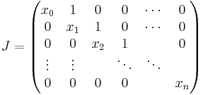
Divided differences of polynomials are particularly interesting, because they can benefit from the Leibniz rule. The matrix $J$ with

$J= \begin{pmatrix} x_0 & 1 & 0 & 0 & \cdots & 0 \\ 0 & x_1 & 1 & 0 & \cdots & 0 \\ 0 & 0 & x_2 & 1 & & 0 \\ \vdots & \vdots & & \ddots & \ddots & \\ 0 & 0 & 0 & 0 & & x_n \end{pmatrix}$

contains the divided difference scheme for the identity function with respect to the nodes $x_0,\dots,x_n$ , thus $J^n$ contains the divided differences for the power function with exponent $n$ . Consequently you can obtain the divided differences for a polynomial function $\varphi(p)$ with respect to the polynomial $p$ by applying $p$ (more precisely: its corresponding matrix polynomial function $\varphi_{\mathrm{M}}(p)$ ) to the matrix $J$ .

$\varphi(p)(\xi) = a_0 %2B a_1\cdot \xi %2B \dots %2B a_n\cdot \xi^n$

$\varphi_{\mathrm{M}}(p)(J) = a_0 %2B a_1\cdot J %2B \dots %2B a_n\cdot J^n$

$= \begin{pmatrix} \varphi(p)[x_0] & \varphi(p)[x_0,x_1] & \varphi(p)[x_0,x_1,x_2] & \ldots & \varphi(p)[x_0,\dots,x_n] \\ 0 & \varphi(p)[x_1] & \varphi(p)[x_1,x_2] & \ldots & \varphi(p)[x_1,\dots,x_n] \\ \vdots & \ddots & \ddots & \ddots & \vdots \\ 0 & \ldots & 0 & 0 & \varphi(p)[x_n] \end{pmatrix}$

This is known as Opitz' formula. ^[1] ^[2]

Now consider increasing the degree of $p$ to infinity, i.e. turn the Taylor polynomial to a Taylor series. Let $f$ be a function which corresponds to a power series. You can compute a divided difference scheme by computing the according matrix series applied to $J$ . If the nodes $x_0,\dots,x_n$ are all equal, then $J$ is a Jordan block and computation boils down to generalizing a scalar function to a matrix function using Jordan decomposition.

Forward differences

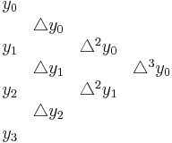
For more details on this topic, see Finite difference.

When the data points are equidistantly distributed we get the special case called forward differences. They are easier to calculate than the more general divided differences.

Definition

Given n data points

$(x_0, y_0),\ldots,(x_{n-1}, y_{n-1})$

with

$x_{\nu} = x_0 %2B \nu h \mbox{ , } h > 0 \mbox{ , } \nu=0,\ldots,n-1$

the divided differences can be calculated via forward differences defined as

$\triangle^{(0)}y_{i}�:= y_{i}$

$\triangle^{(k)}y_{i}�:= \triangle^{(k-1)}y_{i%2B1} - \triangle^{(k-1)}y_{i} \mbox{ , } k \ge 1.$

Example

$\begin{matrix} y_0 & & & \\ & \triangle y_0 & & \\ y_1 & & \triangle^{2} y_0 & \\ & \triangle y_1 & & \triangle^{3} y_0\\ y_2 & & \triangle^{2} y_1 & \\ & \triangle y_2 & & \\ y_3 & & & \\ \end{matrix}$

Computer Program

Java code for Divided differences with GUI by Behzad Torkian

Notes

^ de Boor, Carl, Divided Differences, Surv. Approx. Theory 1 (2005), 46--69
^ Opitz, G. Steigungsmatrizen, Z. Angew. Math. Mech. (1964), 44, T52-T54

Divided differences

Contents

Definition

Notation

Example

Properties

Matrix form

Alternative definitions

Expanded form

Partial fractions

Peano form

Taylor form

First order

Higher order

Polynomials and power series

Forward differences

Definition

Example

Computer Program

Notes

See also