Divergence theorem

Fundamental theorem
Limits of functions
Continuity
Mean value theorem

Differential calculus
Derivative Change of variables Implicit differentiation Taylor's theorem Related rates Rules and identities: Power rule, Product rule, Quotient rule, Chain rule

Integral calculus
Integral Lists of integrals Improper integrals Integration by: parts, disks, cylindrical shells, substitution, trigonometric substitution, partial fractions, changing order

Vector calculus
Gradient Divergence Curl Laplacian Gradient theorem Green's theorem Stokes' theorem Divergence theorem

Multivariable calculus
Matrix calculus Partial derivative Multiple integral Line integral Surface integral Volume integral Jacobian

In vector calculus, the divergence theorem, also known as Ostrogradsky's theorem ^[1], is a result that relates the flow (that is, flux) of a vector field through a surface to the behavior of the vector field inside the surface.

More precisely, the divergence theorem states that the outward flux of a vector field through a closed surface is equal to the volume integral of the divergence of the region inside the surface. Intuitively, it states that the sum of all sources minus the sum of all sinks gives the net flow out of a region.

The divergence theorem is an important result for the mathematics of engineering, in particular in electrostatics and fluid dynamics.

In physics and engineering, the divergence theorem is usually applied in three dimensions. However, it generalizes to any number of dimensions. In one dimension, it is equivalent to the fundamental theorem of calculus.

The theorem is a special case of the more general Stokes' theorem.^[2]

1 Intuition
2 Mathematical statement
- 2.1 Corollaries
3 Example
4 Applications
- 4.1 Differential form and integral form of physical laws
  - 4.1.1 Continuity equations
- 4.2 Inverse-square laws
5 History
6 Examples
7 Notes
8 External links

Intuition

If a fluid is flowing in some area, and we wish to know how much fluid flows out of a certain region within that area, then we need to add up the sources inside the region and subtract the sinks. The fluid flow is represented by a vector field, and the vector field's divergence at a given point describes the strength of the source or sink there. So, integrating the field's divergence over the interior of the region should equal the integral of the vector field over the region's boundary. The divergence theorem says that this is true.

The divergence theorem is thus a conservation law which states that the volume total of all sinks and sources, the volume integral of the divergence, is equal to the net flow across the volume's boundary.^[3]

Mathematical statement

Suppose V is a subset of Rⁿ (in the case of n = 3, V represents a volume in 3D space) which is compact and has a piecewise smooth boundary S. If F is a continuously differentiable vector field defined on a neighborhood of V, then we have

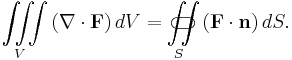
$\iiint\limits_V\left(\nabla\cdot\mathbf{F}\right)dV=\iint\limits_{S}\!\!\!\!\!\!\!\!\!\!\!\subset\!\supset (\mathbf{F}\cdot\mathbf{n})\,dS .$

The left side is a volume integral over the volume V, the right side is the surface integral over the boundary of the volume V. The closed manifold ∂V is quite generally the boundary of V oriented by outward-pointing normals, and n is the outward pointing unit normal field of the boundary ∂V. (dS may be used as a shorthand for n dS.) By the symbol within the two integrals it is stressed once more that ∂V is a closed surface. In terms of the intuitive description above, the left-hand side of the equation represents the total of the sources in the volume V, and the right-hand side represents the total flow across the boundary ∂V.

Corollaries

By applying the divergence theorem in various contexts, other useful identities can be derived (cf. vector identities).

Applying the divergence theorem to the product of a scalar function g and a vector field F, the result is

$\iiint\limits_V\left[\mathbf{F}\cdot \left(\nabla g\right) %2B g \left(\nabla\cdot \mathbf{F}\right)\right] dV = \iint\limits_{S}\!\!\!\!\!\!\!\!\!\!\!\!\!\!\!\!\;\;\;\subset\!\supset g\mathbf{F}\cdot \vec{n} d\mathbf{S}.$

A special case of this is $\scriptstyle \mathbf{F}=\nabla f$ , in which case the theorem is the basis for Green's identities.

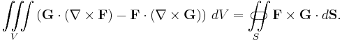
Applying the divergence theorem to the cross-product of two vector fields $\scriptstyle \mathbf{F}\times \mathbf{G}$ , the result is

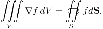
$\iiint\limits_V \left(\mathbf{G}\cdot\left(\nabla\times\mathbf{F}\right) - \mathbf{F}\cdot \left( \nabla\times\mathbf{G}\right)\right)\, dV = \iint\limits_{S}\!\!\!\!\!\!\!\!\!\!\!\!\!\!\!\!\;\;\;\subset\!\supset \mathbf F\times\mathbf{G}\cdot d\mathbf{S}.$

Applying the divergence theorem to the product of a scalar function, f, and a non-zero constant vector, the following theorem can be proven:^[4]

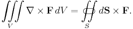
$\iiint\limits_V \nabla f\, dV =\iint\limits_{S}\!\!\!\!\!\!\!\!\!\!\!\!\!\!\!\!\;\;\;\subset\!\supset{f}d \mathbf{S}.$

Applying the divergence theorem to the cross-product of a vector field F and a non-zero constant vector, the following theorem can be proven:^[4]

$\iiint\limits_V \nabla\times\mathbf{F}\, dV = \iint\limits_{S}\!\!\!\!\!\!\!\!\!\!\!\!\!\!\!\!\;\;\;\subset\!\supset{d}\mathbf{S}\times \mathbf{F}.$

Example

Suppose we wish to evaluate

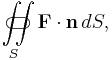
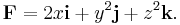
$\iint\limits_{S}\!\!\!\!\!\!\!\!\!\!\!\!\!\!\!\!\;\;\;\subset\!\supset \mathbf{F}\cdot\mathbf{n} \, dS,$

where S is the unit sphere defined by $\scriptstyle x^2%2By^2%2Bz^2=1$ and F is the vector field

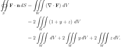
$\mathbf{F} = 2 x\mathbf{i}%2By^2\mathbf{j}%2Bz^2\mathbf{k}.$

The direct computation of this integral is quite difficult, but we can simplify the derivation of the result using the divergence theorem:

$\begin{align} \iint\limits_{S}\!\!\!\!\!\!\!\!\!\!\!\!\!\!\!\!\;\;\;\subset\!\supset \mathbf{F} \cdot \mathbf{n}\,{d}S &= \iiint\limits_W\left(\nabla\cdot\mathbf{F}\right) \, dV\\ &= 2\iiint\limits_W\left(1%2By%2Bz\right) \, dV\\ &= 2\iiint\limits_W \,dV %2B 2\iiint\limits_W y \,dV %2B 2\iiint\limits_W z \,dV. \end{align}$

Since the functions $\scriptstyle y$ and $\scriptstyle z$ are odd on $\scriptstyle S$ (which is a symmetric set with respect to the coordinate planes), one has

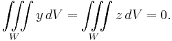
$\iiint\limits_W y\, dV = \iiint\limits_W z\, dV = 0.$

Therefore,

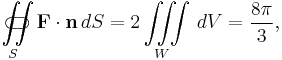
$\iint\limits_{S}\!\!\!\!\!\!\!\!\!\!\!\!\!\!\!\!\;\;\;\subset\!\supset \mathbf{F}\cdot\mathbf{n}\,{d}S = 2\iiint\limits_W \, dV = \frac{8\pi}{3},$

because the unit sphere W has volume $\scriptstyle \frac{4\pi}{3}.$

Applications

Differential form and integral form of physical laws

As a result of the divergence theorem, a host of physical laws can be written in both a differential form (where one quantity is the divergence of another) and an integral form (where the flux of one quantity through a closed surface is equal to another quantity). Three examples are Gauss's law (in electrostatics), Gauss's law for magnetism, and Gauss's law for gravity.

Continuity equations

Main article: continuity equation

Continuity equations offer more examples of laws with both differential and integral forms, related to each other by the divergence theorem. In fluid dynamics, electromagnetism, quantum mechanics, relativity theory, and a number of other fields, there are continuity equations that describe the conservation of mass, momentum, energy, probability, or other quantities. Generically, these equations state that the divergence of the flow of the conserved quantity is equal to the distribution of sources or sinks of that quantity. The divergence theorem states that any such continuity equation can be written in a differential form (in terms of a divergence) and an integral form (in terms of a flux).

Inverse-square laws

Any inverse-square law can instead be written in a Gauss' law-type form (with a differential and integral form, as described above). Two examples are Gauss' law (in electrostatics), which follows from the inverse-square Coulomb's law, and Gauss' law for gravity, which follows from the inverse-square Newton's law of universal gravitation. The derivation of the Gauss' law-type equation from the inverse-square formulation (or vice-versa) is exactly the same in both cases; see either of those articles for details.

History

The theorem was first discovered by Lagrange in 1762, then later independently rediscovered by Gauss in 1813, by Green in 1825 and in 1831 by Ostrogradsky, who also gave the first proof of the theorem. Subsequently, variations on the divergence theorem are correctly called Ostrogradsky's theorem, but also commonly Gauss's theorem, or Green's theorem.

Examples

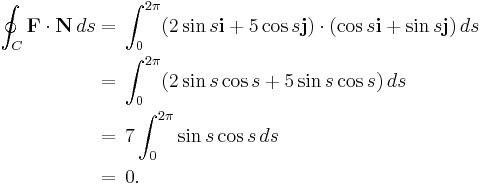
Verify the planar variant of the divergence theorem for a region R, with F(x,y) = 2yi + 5xj, where R is the region bounded by the circle

$\scriptstyle x^2 %2B y^2 = 1.\$

Solution: The boundary of R is the unit circle, C, that can be represented parametrically by:

$x\, = \cos(s);\ y\, = \sin(s)\$

such that $\scriptstyle 0\, \le \,s\, \le \,2\pi$ where s units is the length arc from the point s = 0 to the point P on C. Then a vector equation of C is

$\mathbf{C}(s) = \cos(s)\mathbf{i} %2B \sin(s)\mathbf{j}.\$

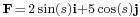At a point $\scriptstyle\mathbf{P}\, = \,(\cos(s),\, \sin(s))$ on C, $\scriptstyle\mathbf{F}\, = \,2\sin(s)\mathbf{i} %2B 5\cos(s)\mathbf{j}$ . Therefore,

$\begin{align}\oint_C \mathbf{F} \cdot \mathbf{N}\, ds &= \,\int_{0}^{2 \pi} ( 2 \sin s \mathbf{i} %2B 5 \cos s \mathbf{j}) \cdot (\cos s \mathbf{i} %2B \sin s \mathbf{j})\, ds\\ &= \,\int_{0}^{2 \pi} (2 \sin s \cos s %2B 5 \sin s \cos s)\, ds\\ &= \,7\int_{0}^{2 \pi} \sin s \cos s\, ds\\ &= \,0.\end{align}\$

Because $\scriptstyle M\, = \,2y\,$ , $\scriptstyle \frac{\partial M}{\partial x} = \,0$ , and because $\scriptstyle N\, = \,5x\,$ , $\scriptstyle \frac{\partial N}{\partial y} = \,0$ . Thus

$\iint\limits_R \, \operatorname{div} \mathbf{F} \,dA = \iint\limits_R \left (\frac{\partial M}{\partial x} %2B \frac{\partial N}{\partial y} \right) \, dA = 0.$

Notes

^ or less correctly as Gauss' theorem (see history for reason)
^ Stewart, James (2008), "Vector Calculus", Calculus: Early Transcendentals (6 ed.), Thomson Brooks/Cole, ISBN 9780495011668
^ Byron, Frederick; Fuller, Robert (1992), Mathematics of Classical and Quantum Physics, Dover Publications, p. 22, ISBN 9780486671642
^ ^a ^b MathWorld

External links

Differential Operators and the Divergence Theorem at MathPages
The Divergence (Gauss) Theorem by Nick Bykov, Wolfram Demonstrations Project.
Weisstein, Eric W., "Divergence Theorem" from MathWorld.

This article was originally based on the GFDL article from PlanetMath at http://planetmath.org/encyclopedia/Divergence.html