Bond duration
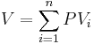
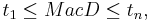
In finance, the duration of a financial asset that consists of fixed cash flows, for example a bond, is the weighted average of the times until those fixed cash flows are received. When an asset is considered as a function of yield, duration also measures the price sensitivity to yield, the rate of change of price with respect to yield or the percentage change in price for a parallel shift in yields. [1] [2]
Since cash flows for bonds are usually fixed, a price change can come from two sources:
- The passage of time (convergence towards par). This is of course totally predictable, and hence not a risk.
- A change in the yield. This can be due to a change in the benchmark yield, and/or change in the yield spread.
The yield-price relationship is inverse, and we would like to have a measure of how sensitive the bond price is to yield changes. A good approximation for bond price changes due to yield is the duration, a measure for interest rate risk. For large yield changes convexity can be added to improve the performance of the duration. A more important use of convexity is that it measures the sensitivity of duration to yield changes. Similar risk measures are used in the options markets are the delta and gamma.
The dual use of the word "duration", as both the weighted average time until repayment and as the percentage change in price, often causes confusion. Strictly speaking, Macaulay duration is the name given to the weighted average time until cash flows are received, and is measured in years. Modified duration is the name given to the price sensitivity and is the percentage change in price for a unit change in yield. When yields are continuously-compounded Macaulay duration and modified duration will be numerically equal. When yields are periodically-compounded Macaulay and modified duration will differ slightly, and in this case there is a simple relation between the two. Modified duration is used more than Macaulay duration.
Macaulay duration and modified duration are both termed "duration" and have the same (or close to the same) numerical value, but it is important to keep in mind the conceptual distinctions between them. Macaulay duration is a time measure with units in years, and really makes sense only for an instrument with fixed cash flows. For a standard bond the Macaulay duration will be between 0 and the maturity of the bond. It is equal to the maturity if and only if the bond is a zero-coupon bond.
Modified duration, on the other hand, is a derivative (rate of change) or price sensitivity and measures the percentage rate of change of price with respect to yield. (Price sensitivity with respect to yields can also be measured in absolute (dollar) terms, and the absolute sensitivity is often referred to as dollar duration, DV01, PV01, or delta (δ or Δ) risk.) The concept of modified duration can be applied to interest-rate sensitive instruments with non-fixed cash flows, and can thus be applied to a wider range of instruments than can Macaulay duration.
For every-day use, the equality (or near-equality) of the values for Macaulay and modified duration can be a useful aid to intuition. For example a standard ten-year coupon bond will have Macaulay duration somewhat but not dramatically less than 10 years and from this we can infer that the modified duration (price sensitivity) will also be somewhat but not dramatically less than 10%. Similarly, a two-year coupon bond will have Macaulay duration somewhat below 2 years, and modified duration somewhat below 2%. (For example a ten-year 5% par bond has a modified duration of 7.8% while a two-year 5% par bond has a modified duration of 1.9%.)
Contents |
Macaulay duration
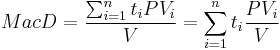
Macaulay duration, named for Frederick Macaulay who introduced the concept, is the weighted average maturity of cash flows. Consider some set of fixed cash flows. The present value of these cash flows is:
Macaulay duration is defined as:[1][2] [3]
- (1)
where:
 indexes the cash flows,
 is the present value of the th cash payment from an asset,
 is the time in years until the th payment will be received,
 is the present value of all cash payments from the asset.
In the second expression the fractional term is the ratio of the cash flow to the total PV. These terms add to 1.0 and serve as weights for a weighted average. Thus the overall expression is a weighted average of time until cash flow payments, with weight  being the proportion of the asset's present value due to cash flow .
For a set of all-positive fixed cash flows the weighted average will fall between 0 (the minimum time), or more precisely  (the time to the first payment) and the time of the final cash flow. The Macaulay duration will equal the final maturity if and only if there is only a single payment at maturity. In symbols, if cash flows are, in order,
  , then:
with the inequalities being strict unless it has a single cash flow. In terms of standard bonds (for which cash flows are fixed and positive), this means the Macaulay duration will equal the bond maturity only for a zero-coupon bond.
Macaulay duration has the diagrammatic interpretation shown in figure 1. This represents the bond discussed in the example below, two year maturity with a coupon of 20% and continuously-compounded yield of 3.9605%. The circles represents the PV of the payments, with the coupon circles getting smaller the further out they are and the final large circle including the final principal repayment. If these circles were put on a balance beam, the fulcrum of the beam would represent the weighted average distance (time to payment), which is 1.78 years in this case.
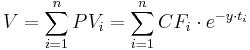
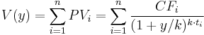
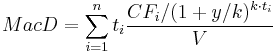
For most practical calculations, the Macaulay duration is calculated using the yield to maturity to calculate the  :
:
- (2)
- (3)
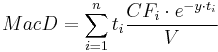
where:
- indexes the cash flows,
- is the present value of the th cash payment from an asset,
 is the cash flow of the th payment from an asset,
 is the yield to maturity (continuously-compounded) for an asset,
- is the time in years until the th payment will be received,
- is the present value of all cash payments from the asset until maturity.
Macaulay gave two alternative measures:
- Expression (1) is Macaulay–Weil duration which uses zero-coupon bond prices as discount factors, and
- Expression (3) which uses the bond's yield to maturity to calculate discount factors.
The key difference between the two is that the Macaulay–Weil duration allows for the possibility of a sloping yield curve, whereas the second form is based on a constant value of the yield , not varying by term to payment. With the use of computers, both forms may be calculated but expression (3), assuming a constant yield, is more widely used because of the application to modified duration.
Modified duration
In contrast to Macaulay duration, modified duration (sometimes abbreviated DM) is a price sensitivity measure, defined as the percentage derivative of price with respect to yield. Modified duration applies when a bond or other asset is considered as a function of yield. In this case one can measure the logarithmic derivative with respect to yield:
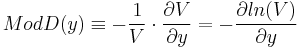
It turns out that when the yield is expressed continuously-compounded, Macaulay duration and modified duration are equal, while for periodically-compounded yields the relation between Macaulay duration and modified duration is:
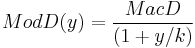
where  is the compounding frequency (1 for annual, 2 for semi-annual, etc.) We can derive this expression from the derivative definition of modified duration above.
First, consider the case of continuously-compounded yields. If we take take the derivative of price or present value, expression (2), with respect to the continuously-compounded yield y we see that:
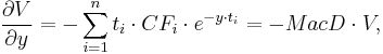
In other words, for yields expressed continuously-compounded, 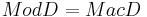 .[1]
.[1]
In financial markets yields are usually expressed periodically-compounded (say annually or semi-annually) instead of continuously-compounded. Then expression (2) becomes:
and expression (3) becomes:
where is the compounding frequency (1 for annual, 2 for semi-annual, etc.) In this case, when we take the derivative of the value with respect to the periodically-compounded yield we find [4]
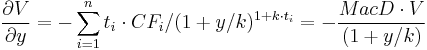
This gives the well-known relation between Macaulay duration and modified duration quoted above. It should be remembered that, even though Macaulay duration and modified duration are closely related, they are conceptually distinct. Macaulay duration is a weighted average time until repayment (measured in units of time such as years) while modified duration is a price sensitivity measure when the price is treated as a function of yield, the percentage change in price with respect to yield.
Units
For modified duration the common units are the percent change in price per one percentage point change in yield per year (for example yield going from 8% per year (y = 0.08) to 9% per year (y = 0.09)). This will give modified duration close to the value of Macaulay duration (and the same when rates are continuously-compounded).
Formally, modified duration is a semi-elasticity, the percent change in price for a unit change in yield, rather than an elasticity, which is a percentage change in output for a percentage change in input. Modified duration is a rate of change, the percent change in price per change in yield.
In derivatives pricing ("The Greeks"), the closest analogous quantity is the λ or Lambda, which is the price elasticity (percentage change in price for percentage change in input), and, unlike modified duration, is an actual elasticity.
Non-Fixed Cash Flows
Modified duration can be extended to instruments with non-fixed cash flows, while Macaulay duration applies only to fixed cash flow instruments. Modified duration is defined as the logarithmic derivative of price with respect to yield, and such a definition will apply to instruments that depend on yields, whether or not the cash flows are fixed.
Finite Yield Changes
Modified duration is defined above as a derivative (as the term relates to calculus) and so is based on infinitesimal changes. Modified duration is also useful as a measure of the sensitivity of a bond's market price to finite interest rate (i.e., yield) movements. For a small change in yield,  ,
,
Thus modified duration is approximately equal to the percentage change in price for a given finite change in yield. So a 15-year bond with a Macaulay duration of 7 years would have a Modified duration of roughly 7% and would fall approximately 7% in value if the interest rate increased by one percentage point (say from 7% to 8%).[5]
Fisher-Weil Duration
Fisher-Weil duration is a refinement of Macaulay’s duration which takes into account the term structure of interest rates.Fisher-Weil duration calculates accordingly the present values of the relevant cashflows (more strictly) by using the zero coupon yield for each respective maturity.
Key rate Duration
Key rate duration measures portfolio sensitivity or bond's price sensitivity to independent shifts along the yield curve at selected “key” points. Key rate duration is calculated value in relation to a 1% change in yield for a given maturity. Duration is the value of a 1% change (100 basis points) in yield for a given maturity.Key Rate Duration calculates the price response separately for a 1% change in each zero-coupon rate used to calculate the PV of the bond. Gives a better picture of which parts of the term-structure is responsible for how much of total interest rate risk. The key rate durations can then be summed up to give an overall interest rate risk measure, comparable with modified duration. Key rate duration is quoted as a percentage or in basis points.
Bond Duration Formulas
For a standard bond with fixed, semi-annual payments the bond duration closed-form formula is:

- FV = par value
- C = coupon payment per period (half-year)
- i = discount rate per period (half-year)
- a = fraction of a period remaining until next coupon payment
- m = number of full coupon periods until maturity
- P = bond price (present value of cash flows discounted with rate i)
For a bond with coupon frequency but an integer number of periods (so that there is no fractional payment period), the formula simplifies to: [6]
![MacD = \left[ \frac {(1%2By/k)}{y/k} - \frac {100(1%2By/k)%2Bm(c/k-100y/k)}{(c/k)[(1%2By/k)^m-1]%2B100y/k} \right ] / k](/2012-wikipedia_en_all_nopic_01_2012/I/c4cf99bd5c06c34db91ac4e4b5b0da25.png)
where
- y = Yield (per year, in decimal form),
- c = Coupon (per year, in percent),
- m = Number of coupon periods.
Example
Consider a 2-year bond with a 20% semi-annual coupon and a yield of 4% semi-annually compounded. The total PV will be:


The Macaulay duration is then
 .
.
The simple formula above gives (y/k =.04/2=.02, c/k = 20/2 = 10):
![MacD = \left[ \frac {(1.02)}{0.02} - \frac {100(1.02)%2B4(10-2)}{10[(1.02)^{4}-1]%2B2} \right] / 2 = 1.777 years](/2012-wikipedia_en_all_nopic_01_2012/I/8dda9cc5b196756e65be0b05bd5ab0ff.png)
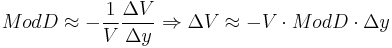
The modified duration, measured as percentage change in price per one percentage point change in yield, is:
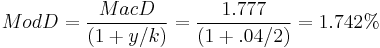 (% change in price per 1 percentage point change in yield)
The DV01, measured as dollar change in price for a $100 nominal bond for a one percentage point change in yield, is
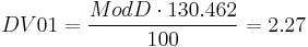 ($ per 1 percentage point change in yield)
where the division by 100 is because modified duration is the percentage change.
Dollar duration, DV01
The dollar duration or DV01 is defined as the derivative of the value with respect to yield:
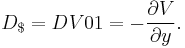
so that it is the product of the modified duration and the price (value):
 ($ per 1 percentage point change in yield)
or
 ($ per 1 basis point change in yield)
The DV01 is analogous to the delta in derivative pricing (The Greeks) – it is the ratio of a price change in output (dollars) to unit change in input (a basis point of yield). Dollar duration or DV01 is the change in price in dollars, not in percentage. It gives the dollar variation in a bond's value per unit change in the yield. It is often measured per 1 basis point - DV01 is short for "dollar value of an 01" (or 1 basis point). The names BPV (basis point value) or PV01 (present value of an 01) are also used, although PV01 more accurately refers to the value of a one dollar or one basis point annuity. (For a par bond and a flat yield curve the DV01, derivative of price w.r.t. yield, and PV01, value of a one-dollar annuity, will actually have the same value.)
DV01 or dollar duration can be used for instruments with zero up-front value such as interest rate swaps where percentage changes and modified duration are less useful.
Application to VaR
Dollar duration  is commonly used for VaR (Value-at-Risk) calculation. To illustrate applications to portfolio risk management, consider a portfolio of securities dependent on the interest rates
  as risk factors, and let
denote the value of such portfolio. Then the exposure vector  has components
Accordingly, the change in value of the portfolio can be approximated as
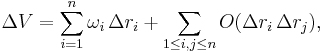
that is, a component that is linear in the interest rate changes plus an error term which is at least quadratic. This formula can be used to calculate the VaR of the portfolio by ignoring higher order terms. Typically cubic or higher terms are truncated. Quadratic terms, when included, can be expressed in terms of (multi-variate) bond convexity. One can make assumptions about the joint distribution of the interest rates and then calculate VaR by Monte Carlo simulation or, in some special cases (e.g., Gaussian distribution assuming a linear approximation), even analytically. The formula can also be used to calculate the DV01 of the portfolio (cf. below) and it can be generalized to include risk factors beyond interest rates.
Embedded options and effective duration
For bonds that have embedded options, such as putable and callable bonds, Macaulay duration will not correctly approximate the price move for a change in yield.
To price such bonds, one must use option pricing to determine the value of the bond, and then one can compute its delta (and hence its lambda), which is the duration. The effective duration is a discrete approximation to this latter, and depends on an option pricing model.
Consider a bond with an embedded put option. As an example, a $1,000 bond that can be redeemed by the holder at par at any time before the bond's maturity (i.e. an American put option). No matter how high interest rates become, the price of the bond will never go below $1,000 (ignoring counterparty risk). This bond's price sensitivity to interest rate changes is different from a non-puttable bond with otherwise identical cashflows. Bonds that have embedded options can be analyzed using "effective duration". Effective duration is a discrete approximation of the slope of the bond's value as a function of the interest rate.
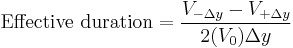
where Δ y is the amount that yield changes, and
are the values that the bond will take if the yield falls by y or rises by y, respectively. However this value will vary depending on the value used for Δ y.
Spread duration
Sensitivity of a bond's market price to a change in Option Adjusted Spread (OAS). Thus the index, or underlying yield curve, remains unchanged.
Average duration
The sensitivity of a portfolio of bonds such as a bond mutual fund to changes in interest rates can also be important. The average duration of the bonds in the portfolio is often reported. The duration of a portfolio equals the weighted average maturity of all of the cash flows in the portfolio. If each bond has the same yield to maturity, this equals the weighted average of the portfolio's bond's durations, with weights proportional to the bond prices.[1] Otherwise the weighted average of the bond's durations is just a good approximation, but it can still be used to infer how the value of the portfolio would change in response to changes in interest rates.
Convexity
Duration is a linear measure of how the price of a bond changes in response to interest rate changes. As interest rates change, the price does not change linearly, but rather is a convex function of interest rates. Convexity is a measure of the curvature of how the price of a bond changes as the interest rate changes. Specifically, duration can be formulated as the first derivative of the price function of the bond with respect to the interest rate in question, and the convexity as the second derivative.
Convexity also gives an idea of the spread of future cashflows. (Just as the duration gives the discounted mean term, so convexity can be used to calculate the discounted standard deviation, say, of return.)
Note that convexity can be both positive and negative. A bond with positive convexity will not have any call features - i.e. the issuer must redeem the bond at maturity - which means that as rates fall, its price will rise.
On the other hand, a bond with call features - i.e. where the issuer can redeem the bond early - is deemed to have negative convexity, which is to say its price should fall as rates fall. This is because the issuer can redeem the old bond at a high coupon and re-issue a new bond at a lower rate, thus providing the issuer with valuable optionality.
Mortgage-backed securities (pass-through mortgage principal prepayments) with US-style 15- or 30-year fixed rate mortgages as collateral are examples of callable bonds.
See also
- Bond convexity
- Bond valuation
- Immunization (finance)
- Stock duration
- Bond duration closed-form formula
- Yield to maturity
- Day count convention
Lists
Notes
References
- ^ a b c d Hull, John C. (1993), Options, Futures, and Other Derivative Securities (Second ed.), Englewood Cliffs, NJ: Prentice-Hall, Inc., pp. 99–101
- ^ a b Brealey, Richard A.; Myers, Stewart C.; Allen, Franklin (2011), Principles of Corporate Finance (Tenth ed.), New York, NY: McGraw-Hill Irwin, pp. 50–53
- ^ Marrison, Chris (2002), The Fundamentals of Risk Measurement, Boston, MA: McGraw-Hill, pp. 57–58
- ^ Berk, Jonathan; DeMarzo, Peter (2011), Corporate Finance (Second ed.), Boston, MA: Prentice Hall, pp. 966–969
- ^ "Macaulay Duration" by Fiona Maclachlan, The Wolfram Demonstrations Project.
- ^ Bodie; Kane; Marcus (1993), Investments (Second ed.), p. 478
External links
- Investopedia’s duration explanation
- Hussman Funds - Weekly Market Comment: February 23, 2004 - Buy-and-Hold For the Duration?
- Online duration, price and yield calculator with graphics
- Online real-time Bond Price, Duration, and Convexity Calculator, by Razvan Pascalau, Univ. of Alabama
- Riskglossary.com for a good explanation on the multiple definitions of duration and their origins.
- Modified duration calculator
- Bond Yield Duration and Convexity Calculator Financial Technology Laboratories
|
|||||||||||||||||||||||