Covariance
In probability theory and statistics, covariance is a measure of how much two random variables change together. If the greater values of one variable mainly correspond with the greater values of the other variable, and the same holds for the smaller values, i.e. the variables tend to show similar behavior, the covariance is a positive number. In the opposite case, when the greater values of one variable mainly correspond to the smaller values of the other, i.e. the variables tend to show opposite behavior, the covariance is negative. The sign of the covariance therefore shows the tendency in the linear relationship between the variables. The magnitude of the covariance is not that easy to interpret. The normalized version of the covariance, the correlation coefficient, however shows by its magnitude the strength of the linear relation.
A distinction has to be made between the covariance of two random variables, a population parameter, that can be seen as a property of the joint probability distribution at one side, and on the other side the sample covariance, which serves as an estimated value of the parameter.
Contents |
Definition
The covariance between two jointly distributed real-valued random variables X and Y with finite second moments is
![\operatorname{Cov}(X,Y) = \operatorname{E}{\big[(X - \operatorname{E}[X])(Y - \operatorname{E}[Y])\big]}](/2012-wikipedia_en_all_nopic_01_2012/I/4a466dd2899716974897e36455d3d0a8.png)
where E[X] is the expected value of X. By using some properties of expectations, this can be simplified to
![\operatorname{Cov}(X,Y) = \operatorname{E}\big[X Y\big] - \operatorname{E}[X]\operatorname{E}[Y]](/2012-wikipedia_en_all_nopic_01_2012/I/247e4181ebc7e3aabfb042a7619c897a.png)
For random vectors X and Y (of dimension m and n respectively) the m×n covariance matrix is equal to
![\begin{align}
\operatorname{Cov}(X,Y)
& = \operatorname{E}\left[(X - \operatorname{E}[X])(Y - \operatorname{E}[Y])^T\right]\\
& = \operatorname{E}\left[X Y^T\right] - \operatorname{E}[X]\operatorname{E}[Y]^T
\end{align}](/2012-wikipedia_en_all_nopic_01_2012/I/d1a4014f2af0237786990806bda25807.png)
where MT is the transpose of a matrix (or vector) M.
The (i,j)-th element of this matrix is equal to the covariance Cov(Xi, Yj) between the i-th scalar component of X and the j-th scalar component of Y. In particular, Cov(Y, X) is the transpose of Cov(X, Y).
Random variables whose covariance is zero are called uncorrelated.
The units of measurement of the covariance Cov(X, Y) are those of X times those of Y. By contrast, correlation, which depends on the covariance, is a dimensionless measure of linear dependence.
Properties
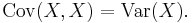
- Variance is a special case of the covariance when the two variables are identical:
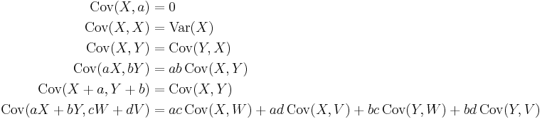
- If X, Y, W, and V are real-valued random variables and a, b, c, d are constant ("constant" in this context means non-random), then the following facts are a consequence of the definition of covariance:
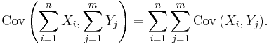
For sequences X1, ..., Xn and Y1, ..., Ym of random variables, we have
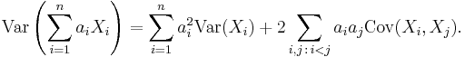
For a sequence X1, ..., Xn of random variables, and constants a1, ..., an, we have
If X and Y are independent, then their covariance is zero. This follows because under independence,
![\operatorname{E}\left[X \cdot Y\right] = E[X] \cdot E[Y].](/2012-wikipedia_en_all_nopic_01_2012/I/e8a7312ffe800c729a666a22bcd39a22.png)
The converse, however, is not generally true. For example, let X be uniformly distributed in [-1, 1] and let Y = X2. Clearly, X and Y are dependent, but
![\begin{align}
\operatorname{Cov}(X, Y) &= \operatorname{Cov}(X, X^2) \\
&= \operatorname{E}\!\left[X \cdot X^2\right] - \operatorname{E}[X] \cdot \operatorname{E}\!\left[X^2\right] \\
&= \operatorname{E}\!\left[X^3\right] - \operatorname{E}[X]\operatorname{E}\!\left[X^2\right] \\
&= 0 - 0 \cdot \operatorname{E}\!\left[X^2\right] \\
&= 0.
\end{align}](/2012-wikipedia_en_all_nopic_01_2012/I/d52ef425baf9e727fc5449eb83c0631b.png)
Relationship to inner products
Many of the properties of covariance can be extracted elegantly by observing that it satisfies similar properties to those of an inner product:
- bilinear: for constants a and b and random variables X, Y, and U, Cov(aX + bY, U) = a Cov(X, U) + b Cov(Y, U)
- symmetric: Cov(X, Y) = Cov(Y, X)
- positive semi-definite: Var(X) = Cov(X, X) ≥ 0, and Cov(X, X) = 0 implies that X is a constant random variable (K).
In fact these properties imply that the covariance defines an inner product over the quotient vector space obtained by taking the subspace of random variables with finite second moment and identifying any two that differ by a constant. (This identification turns the positive semi-definiteness above into positive definiteness.) That quotient vector space is isomorphic to the subspace of random variables with finite second moment and mean zero; on that subspace, the covariance is exactly the L2 inner product of real-valued functions on the sample space.
As a result for random variables with finite variance the following inequality holds via the Cauchy–Schwarz inequality:

Proof: If Var(Y) = 0, then it holds trivially. Otherwise, let random variable
Then we have:
![\begin{align}
0 \le \operatorname{Var}(Z) & = \operatorname{Cov}\left(X - \frac{\operatorname{Cov}(X,Y)}{\operatorname{Var}(Y)} Y,X - \frac{\operatorname{Cov}(X,Y)}{\operatorname{Var}(Y)} Y \right) \\[12pt]
& = \operatorname{Var}(X) - \frac{ (\operatorname{Cov}(X,Y))^2 }{\operatorname{Var}(Y)}
\end{align}](/2012-wikipedia_en_all_nopic_01_2012/I/51f2ca6f736e698c98668426150c19ee.png)
QED.
Calculating the sample covariance
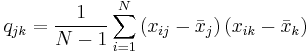
The sample covariance of N observations of K variables is the K-by-K matrix ![\textstyle \mathbf{Q}=\left[ q_{jk}\right]](/2012-wikipedia_en_all_nopic_01_2012/I/932f8f4588aa1865a50de9e7dcd9a8cf.png) with the entries given by
with the entries given by
The sample mean and the sample covariance matrix are unbiased estimates of the mean and the covariance matrix of the random vector  , a row vector whose jth element (j = 1, ..., K) is one of the random variables. The reason the sample covariance matrix has
  in the denominator rather than
  is essentially that the population mean
  is not known and is replaced by the sample mean
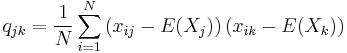
  . If the population mean is known, the analogous unbiased estimate is given by
Comments
The covariance is sometimes called a measure of "linear dependence" between the two random variables. That does not mean the same thing as in the context of linear algebra (see linear dependence). When the covariance is normalized, one obtains the correlation matrix. From it, one can obtain the Pearson coefficient, which gives us the goodness of the fit for the best possible linear function describing the relation between the variables. In this sense covariance is a linear gauge of dependence.
See also
- Covariance function
- Covariance matrix
- Covariance operator
- Correlation
- Eddy covariance
- Law of total covariance
- Autocovariance
- Analysis of covariance
- Algorithms for calculating variance#Covariance
References
External links
|
|||||||||||||||||||||||||||||||||||||||||||||||||||||||||||||||||||||||||||||||||||||||||||||||||||||||||||||||||||||||||||||||||||||||||||