Conditional expectation

In probability theory, a conditional expectation (also known as conditional expected value or conditional mean) is the expected value of a real random variable with respect to a conditional probability distribution.

The concept of conditional expectation is extremely important in Kolmogorov's measure-theoretic definition of probability theory. In fact, the concept of conditional probability itself is actually defined in terms of conditional expectation.

1 Introduction
2 Formal definition
- 2.1 Discussion
3 Definition of conditional probability
4 Conditioning as factorization
5 Conditioning relative to a subalgebra
6 Basic properties
7 See also
8 Notes
9 References
10 External links

Introduction

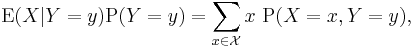
Let X and Y be discrete random variables, then the conditional expectation of X given the event Y=y is a function of y over the range of Y

$\operatorname{E} (X | Y=y ) = \sum_{x \in \mathcal{X}} x \ \operatorname{P}(X=x|Y=y) = \sum_{x \in \mathcal{X}} x \ \frac{\operatorname{P}(X=x,Y=y)}{\operatorname{P}(Y=y)},$

where $\mathcal{X}$ is the range of X.

A problem arises when we attempt to extend this to the case where Y is a continuous random variable. In this case, the probability P(Y=y) = 0, and the Borel–Kolmogorov paradox demonstrates the ambiguity of attempting to define conditional probability along these lines.

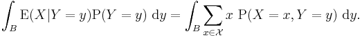
However the above expression may be rearranged:

$\operatorname{E} (X | Y=y) \operatorname{P}(Y=y) = \sum_{x \in \mathcal{X}} x \ \operatorname{P}(X=x,Y=y),$

and although this is trivial for individual values of y (since both sides are zero), it should hold for any measurable subset B of the domain of Y that:

$\int_B \operatorname{E} (X | Y=y) \operatorname{P}(Y=y) \ \operatorname{d}y = \int_B \sum_{x \in \mathcal{X}} x \ \operatorname{P}(X=x,Y=y) \ \operatorname{d}y.$

In fact, this is a sufficient condition to define both conditional expectation, and conditional probability.

Formal definition

Let $\scriptstyle (\Omega, \mathcal A, \operatorname{P})$ be a probability space, with a real random variable X and a sub-σ-algebra $\scriptstyle \mathcal B \subseteq \mathcal A$ . Then a conditional expectation of X given $\scriptstyle \mathcal B$ is any $\scriptstyle \mathcal B$ -measurable function $\scriptstyle \operatorname{E}(X|\mathcal{B}):\Omega \to \mathbb{R}$ which satisfies:

$\int_B \operatorname{E}(X|\mathcal{B}) (\omega) \ \operatorname{d} \operatorname{P}(\omega) = \int_B X(\omega) \ \operatorname{d} \operatorname{P}(\omega) \qquad \text{for each} \quad B \in \mathcal{B}$ .^[1]

Note that $\scriptstyle \operatorname{E}(X|\mathcal{B})$ is simply the name of the conditional expectation function.

Discussion

A couple of points worth noting about the definition:

This is not a constructive definition; we are merely given the required property that a conditional expectation must satisfy.
- The required property has the same form as the last expression in the Introduction section.
- Existence of a conditional expectation function is determined by the Radon–Nikodym theorem, a sufficient condition is that the (unconditional) expected value for X exist.
- Uniqueness can be shown to be almost sure: that is, versions of the same conditional expectation will only differ on a set of probability zero.
The σ-algebra controls the "granularity" of the conditioning. A conditional expectation over a finer-grained σ-algebra will allow us to condition on a wider variety of events.
- To condition freely on values of a random variable Y with state space $\scriptstyle (\mathcal Y, \Sigma)$ , it suffices to define the conditional expectation using the pre-image of Σ with respect to Y:

$\mathcal{B} = \sigma(Y):= Y^{-1}\left(\Sigma\right):= \{Y^{-1}(S)�: S \in \Sigma \}$

This suffices to ensure that the conditional expectation is σ(Y)-measurable. Although conditional expectation is defined to condition on events in the underlying probability space Ω, the requirement that it be σ(Y)-measurable allows us to condition on $\mathcal{Y}$ as in the introduction.

Definition of conditional probability

For any event $A \in \mathcal{A} \supseteq \mathcal B$ , define the indicator function:

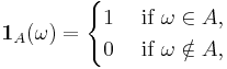
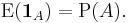
$\mathbf{1}_A (\omega) = \begin{cases} 1 \; &\text{if } \omega \in A, \\ 0 \; &\text{if } \omega \notin A, \end{cases}$

which is a random variable with respect to the Borel σ-algebra on (0,1). Note that the expectation of this random variable is equal to the probability of A itself:

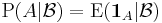
$\operatorname{E}(\mathbf{1}_A) = \operatorname{P}(A). \;$

Then the conditional probability given $\scriptstyle \mathcal B$ is a function 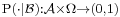$\scriptstyle \operatorname{P}(\cdot|\mathcal{B}):\mathcal{A} \times \Omega \to (0,1)$ such that $\scriptstyle \operatorname{P}(A|\mathcal{B})$ is the conditional expectation of the indicator function for A:

$\operatorname{P}(A|\mathcal{B}) = \operatorname{E}(\mathbf{1}_A|\mathcal{B}) \;$

In other words, $\scriptstyle \operatorname{P}(A|\mathcal{B})$ is a $\scriptstyle \mathcal B$ -measurable function satisfying

$\int_B \operatorname{P}(A|\mathcal{B}) (\omega) \, \operatorname{d} \operatorname{P}(\omega) = \operatorname{P} (A \cap B) \qquad \text{for all} \quad A \in \mathcal{A}, B \in \mathcal{B}.$

A conditional probability is regular if $\scriptstyle \operatorname{P}(\cdot|\mathcal{B})(\omega)$ is also a probability measure for all ω ∈ Ω. An expectation of a random variable with respect to a regular conditional probability is equal to its conditional expectation.

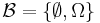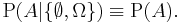
For the trivial sigma algebra $\mathcal B= \{\emptyset,\Omega\}$ the conditional probability is a constant function, $\operatorname{P}\!\left( A| \{\emptyset,\Omega\} \right) \equiv\operatorname{P}(A).$

For $A\in \mathcal{B}$ , as outlined above, $\operatorname{P}(A|\mathcal{B})=1_A.$ .

Conditioning as factorization

In the definition of conditional expectation that we provided above, the fact that Y is a real random variable is irrelevant: Let U be a measurable space, that is, a set equipped with a σ-algebra $\Sigma$ of subsets. A U-valued random variable is a function $Y\colon (\Omega,\mathcal A) \mapsto (U,\Sigma)$ such that $Y^{-1}(B)\in \mathcal A$ for any measurable subset $B\in \Sigma$ of U.

We consider the measure Q on U given as above: Q(B) = P(Y⁻¹(B)) for every measurable subset B of U. Then Q is a probability measure on the measurable space U defined on its σ-algebra of measurable sets.

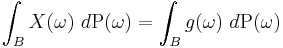
Theorem. If X is an integrable random variable on Ω then there is one and, up to equivalence a.e. relative to Q, only one integrable function g on U (which is written $g= \operatorname{E}(X \mid Y)$ ) such that for any measurable subset B of U:

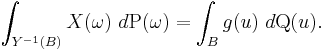
$\int_{Y^{-1}(B)} X(\omega) \ d \operatorname{P}(\omega) = \int_{B} g(u) \ d \operatorname{Q} (u).$

There are a number of ways of proving this; one as suggested above, is to note that the expression on the left hand side defines, as a function of the set B, a countably additive signed measure μ on the measurable subsets of U. Moreover, this measure μ is absolutely continuous relative to Q. Indeed Q(B) = 0 means exactly that Y⁻¹(B) has probability 0. The integral of an integrable function on a set of probability 0 is itself 0. This proves absolute continuity. Then the Radon–Nikodym theorem provides the function g, equal to the density of μ with respect to Q.

The defining condition of conditional expectation then is the equation

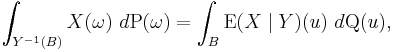
$\int_{Y^{-1}(B)} X(\omega) \ d \operatorname{P}(\omega) = \int_{B} \operatorname{E}(X \mid Y)(u) \ d \operatorname{Q} (u),$

and it holds that

$\operatorname{E}(X \mid Y) \circ Y= \operatorname{E}\left(X \mid Y^{-1} \left(\Sigma\right)\right).$

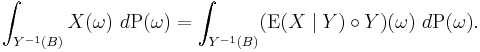
We can further interpret this equality by considering the abstract change of variables formula to transport the integral on the right hand side to an integral over Ω:

$\int_{Y^{-1}(B)} X(\omega) \ d \operatorname{P}(\omega) = \int_{Y^{-1}(B)} (\operatorname{E}(X \mid Y) \circ Y)(\omega) \ d \operatorname{P} (\omega).$

This equation can be interpreted to say that the following diagram is commutative in the average.

                  E(X|Y)= goY
Ω  ───────────────────────────> R
          Y                        g=E(X|Y= ·)
Ω  ──────────>   R    ───────────> R
  
ω  ──────────> Y(ω)  ───────────> g(Y(ω)) = E(X|Y=Y(ω))
  
                        y    ───────────> g(  y ) = E(X|Y=  y )

The equation means that the integrals of X and the composition 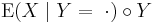$\operatorname{E}(X \mid Y=\ \cdot)\circ Y$ over sets of the form Y⁻¹(B), for B a measurable subset of U, are identical.

Conditioning relative to a subalgebra

There is another viewpoint for conditioning involving σ-subalgebras N of the σ-algebra M. This version is a trivial specialization of the preceding: we simply take U to be the space Ω with the σ-algebra N and Y the identity map. We state the result:

Theorem. If X is an integrable real random variable on Ω then there is one and, up to equivalence a.e. relative to P, only one integrable function g such that for any set B belonging to the subalgebra N

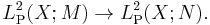
$\int_{B} X(\omega) \ d \operatorname{P}(\omega) = \int_{B} g(\omega) \ d \operatorname{P} (\omega)$

where g is measurable with respect to N (a stricter condition than the measurability with respect to M required of X). This form of conditional expectation is usually written: E(X|N). This version is preferred by probabilists. One reason is that on the space of square-integrable real random variables (in other words, real random variables with finite second moment) the mapping X → E(X|N) is self-adjoint

$\operatorname E(X\cdot\operatorname E(Y|N)) = \operatorname E\left(\operatorname E(X|N)\cdot \operatorname E(Y|N)\right) = \operatorname E(\operatorname E(X|N)\cdot Y)$

and an orthogonal projection

$L^2_{\operatorname{P}}(X;M) \rightarrow L^2_{\operatorname{P}}(X;N).$

Basic properties

Let (Ω, M, P) be a probability space, and let N be a σ-subalgebra of M.

Conditioning with respect to N is linear on the space of integrable real random variables.

$\operatorname{E}(1|N) = 1.$ More generally, $\operatorname{E} (Y|N)= Y$ for every integrable N–measurable random variable Y on Ω.

$\operatorname{E}(1_B \, \operatorname{E} (X|N))= \operatorname{E}(1_B \, X)$ for all B ∈ N and every integrable random variable X on Ω.

Jensen's inequality holds: If ƒ is a convex function, then

$f(\operatorname{E}(X \mid N) ) \leq \operatorname{E}(f \circ X \mid N).$

Conditioning is a contractive projection

$L^s_P(\Omega; M) \rightarrow L^s_P(\Omega; N), \text{ i.e. } \operatorname{E}|\operatorname{E}(X|N)|^s \le \operatorname{E}|X|^s$

for any s ≥ 1.

Notes

^ Loève (1978), p. 7

References

Kolmogorov, Andrey (1933) (in German). Grundbegriffe der Wahrscheinlichkeitsrechnung. Berlin: Julius Springer.
- Translation: Kolmogorov, Andrey (1956). Foundations of the Theory of Probability (2nd ed.). New York: Chelsea. ISBN 0828400237. http://www.mathematik.com/Kolmogorov/index.html.
Loève, Michel (1978). "Chapter 27. Concept of Conditioning". Probability Theory vol. II (4th ed.). Springer. ISBN 0387902627.
William Feller, An Introduction to Probability Theory and its Applications, vol 1, 1950
Paul A. Meyer, Probability and Potentials, Blaisdell Publishing Co., 1966
Grimmett, Geoffrey; Stirzaker, David (2001). Probability and Random Processes (3rd ed.). Oxford University Press. ISBN 0198572220.

External links

Ushakov, N.G. (2001), "Conditional mathematical expectation", in Hazewinkel, Michiel, Encyclopedia of Mathematics, Springer, ISBN 978-1556080104, http://www.encyclopediaofmath.org/index.php?title=c/c024500