Cobb–Douglas production function

In economics, the Cobb–Douglas functional form of production functions is widely used to represent the relationship of an output to inputs. Similar functions were originally used by Knut Wicksell (1851–1926), while the Cobb-Douglas form was developed and tested against statistical evidence by Charles Cobb and Paul Douglas during 1900–1947.

1 Formulation
2 History
3 Difficulties and criticisms
- 3.1 Dimensional analysis
- 3.2 Lack of microfoundations
4 Some applications
5 Various representations of the production function
- 5.1 Translog (transcendental logarithmic) production function
6 Derived from a CES function
7 See also
8 References
9 External links

Formulation

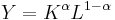
In its most standard form for production of a single good with two factors, the function is

$Y=AL^{\alpha}K^{\beta} \,$

where:

Y = total production (the monetary value of all goods produced in a year)
L = labor input
K = capital input
A = total factor productivity
α and β are the output elasticities of labor and capital, respectively. These values are constants determined by available technology.

Output elasticity measures the responsiveness of output to a change in levels of either labor or capital used in production, ceteris paribus. For example if α = 0.15, a 1% increase in labor would lead to approximately a 0.15% increase in output.

Further, if:

α + β = 1,

the production function has constant returns to scale: Doubling capital K and labour L will also double output Y. If

α + β < 1,

returns to scale are decreasing, and if

α + β > 1

returns to scale are increasing. Assuming perfect competition and α + β = 1, α and β can be shown to be labor and capital's share of output.

Cobb and Douglas were influenced by statistical evidence that appeared to show that labor and capital shares of total output were constant over time in developed countries; they explained this by statistical fitting least-squares regression of their production function. There is now doubt over whether constancy over time exists.

History

Paul Douglas explains that his first formulation of the Cobb–Douglas production function was developed in 1927, when seeking a functional form to relate estimates he had calculated for workers and capital, he spoke with mathematician and colleague Charles Cobb who suggested a function of the form 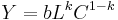$Y = bL^kC^{1-k}$ previously used by Knut Wicksell . Estimating this using least squares, he obtained a result for the marginal productivity of labour (k) to 0.75$ --- which was subsequently confirmed by the National Bureau of Economic Research to be %74.1. Later work in the 1940s prompted them to allow for the exponents on C and L vary, resulting in estimates that subsequently proved to be very close to improved measure of productivity developed at that time.^[1]

A major criticism at the time was that estimates of the production function, although seemingly accurate, were based on such sparse data that it was hard to give them much credibility. Douglas' remarked "I must admit I was discouraged by this criticism and thought of giving up the effort, but there was something which told me I should hold on."^[1] The breakthrough came in using US census data, which was cross sectional and provided a large number of observations. Douglas presented the results of these findings, along with those for other countries, at his 1947 address as president of the American Economic Association. Shortly afterwards, Douglas went into politics and was stricken by ill health --- resulting in little further development on his side. However, two decades later, his production function was widely used, being adopted by economists such as Paul Samuelson and Solow.^[1] The Cobb–Douglas production function is especially notable for being the first time an aggregate or economy-wide production function had been developed, estimated, and the presented to the profession for analysis; it marked a landmark change in how economists approached macroeconomics.^[2]

Difficulties and criticisms

Dimensional analysis

The Cobb–Douglas model is criticized by some Austrian economists such as William Barnett II on the basis of dimensional analysis. They argue it does not having meaningful or economically reasonable units of measurement unless $\alpha %2B \beta = 1$ .^[3] However, other economists in reply to Barnett have argued that the units used are not fundamentally more unnatural than other units commonly used in physics such a log temperature or distance squared.^[4]

Lack of microfoundations

The Cobb–Douglas production function was not developed on the basis of any knowledge of engineering, technology, or management of the production process. It was instead developed because it had attractive mathematical characteristics, such as diminishing marginal returns to either factor of production and the property that expenditure on any given input is a constant fraction of total cost. Crucially, there are no microfoundations for it. In the modern era, economists try to build models up from individual agents acting, rather than imposing a functional form on an entire economy. However, many modern authors have developed models which give Cobb–Douglas production function from the micro level; many New Keynesian models, for example.^[5] It is nevertheless a mathematical mistake to assume that just because the Cobb–Douglas function applies at the micro-level, it also always applies at the macro-level. Similarly, it is not necessarily the case that a macro Cobb–Douglas applies at the disaggregated level. An early microfoundation of the aggregate Cobb–Douglas technology based on linear activities is derived in Houthakker (1955).^[6]

Some applications

Nonetheless, the Cobb–Douglas function has been applied to many other contexts besides production. It can be applied to utility^[7] as follows: U(x₁,x₂)=x₁^αx₂^β; where x₁ and x₂ are the quantities consumed of good #1 and good #2.

In its generalized form, where x₁, x₂, ... ,x_L are the quantities consumed of good #1, good #2, ..., good #L, a utility function representing the Cobb–Douglas preferences may be written as:

$\tilde{u}(x)=\prod_{i=1}^L x_i^{\lambda_{i}}$

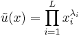
with x = (x₁, x₂, ... ,x_L). Setting $\lambda=\lambda_1%2B\lambda_2%2B...%2B\lambda_L$ and because the function $x \mapsto x^\frac1\lambda$ is strictly monotone for x > 0, it follows that 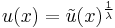$u(x)=\tilde{u}(x)^{\frac1\lambda}$ represents the same preferences. Setting $\alpha_i ={\lambda_i}/\lambda$ it can be shown that 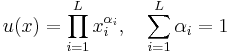$u(x)=\prod_{i=1}^L x_i^{\alpha_{i}}, \quad \sum_{i=1}^L\alpha_{i}=1$ The utility may be maximized by looking at the logarithm of the utility 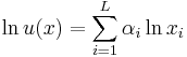$\ln u(x)=\sum_{i=1}^L {\alpha_{i}}\ln x_i$ which makes the consumer's optimization problem:

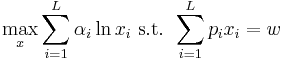
$\max_x \sum_{i=1}^L {\alpha_{i}}\ln x_i \text{ s.t. } \sum_{i=1}^L p_i x_i= w$

This has the solution that:

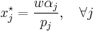
$x_j^\star=\frac{w \alpha_j}{p_j},\quad \forall j$

which has the interpretation that the per-unit fraction of the consumers incomes used in purchasing good j is exactly the marginal term $\alpha_j$

Various representations of the production function

The Cobb–Douglas function form can be estimated as a linear relationship using the following expression:

$\log_e(Y) = a_0 %2B \sum_i{a_i \log_e(I_i)}$

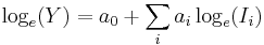
Where:

Y = Output
I_i = Inputs
a_i = model coefficients

The model can also be written as

$Y = (I_1)^{a_1} * (I_2)^{a_2} \cdots$

As noted, the common Cobb–Douglas function used in macroeconomic modeling is

$Y = K^\alpha L^{1-\alpha}$

where K is capital and L is labor. When the model coefficients sum to one, as in this example, the production function is first-order homogeneous, which implies constant returns to scale, that is, if all inputs are scaled by a common factor greater than zero, output will be scaled by the same factor.

Translog (transcendental logarithmic) production function

The translog production function is a generalization of the Cobb–Douglas production function. The name translog stands for 'transcendental logarithmic'.

The three factor translog production function is:

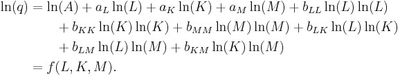
$\begin{align} \ln(q) & = \ln(A) %2B a_L\ln(L) %2B a_K\ln(K) %2B a_M\ln(M) %2B b_{LL}\ln(L)\ln(L) \\ & {} \qquad {} %2Bb_{KK}\ln(K)\ln(K) %2B b_{MM}\ln(M)\ln(M) %2B b_{LK}\ln(L)\ln(K) \\ & {} \qquad {} %2B b_{LM}\ln(L)\ln(M) %2B b_{KM}\ln(K)\ln(M) \\ & = f(L,K,M). \end{align}$

where L = labor, K = capital, M = materials and supplies, and q = product.

Derived from a CES function

Constant elasticity of substitution (CES) function: $Y = A[\alpha K^\gamma %2B (1-\alpha) L^\gamma]^{\frac{1}{\gamma}}$

$\gamma = 0$ corresponds to a Cobb–Douglas function, $Y=AK^\alpha L^{1-\alpha}$

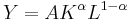
Proof:

$\ln(Y) = \ln(A) %2B \frac{\ln[\alpha K^\gamma %2B (1-\alpha) L^\gamma]}{\gamma}$

Apply l'Hôpital's rule: $\lim_{\gamma\rightarrow 0} \ln(Y) = \ln(A) %2B \alpha \ln(K) %2B (1-\alpha) \ln(L)$

Therefore, $Y=AK^\alpha L^{1-\alpha}$

References

^ ^a ^b ^c "The Cobb-Douglas Production Function Once Again: Its History, Its Testing, and Some New Empirical Values". Journal of Political Economy 84 (5): 903–916. October 1976.
^ Jesus Filipe and Gerard Adams (2005). "The Estimation of the Cobb Douglas Function". Eastern Economic Journal 31 (3): 427–445.
^ (Barnett 2007, p. 96)
^ (Barnett 2007, p. 102)
^ Walsh, Carl (2003). Monetary Theory and Policy (2nd ed.). Cambridge: MIT Press.
^ Houthakker, H.S. (1955), "The Pareto Distribution and the Cobb–Douglas Production Function in Activity Analysis", The Review of Economic Studies 23 (1): 27–31
^ Brenes, Adrián (2011). Cobb-Douglas Utility Function. http://www.wiziq.com/tutorial/160571-Cobb-Douglas-Utility-Function.

Barnett (2007). "Dimensions and Economics: Some Problems". Quarterly Journal of Austrian Economics 7 (1). http://mises.org/journals/qjae/pdf/qjae7_1_10.pdf.
Cobb, C. W.; Douglas, P. H. (1928). "A Theory of Production". American Economic Review 18 (Supplement): 139–165.

External links

Economics

Macroeconomics	Adaptive expectations · Aggregate demand · Balance of payments · Business cycle · Capital flight · Capacity utilization · Central bank · Consumer confidence · Currency · Demand shock · DSGE · Economic indicator · Effective demand · General Theory of Keynes · Great Depression · Growth · Hyperinflation · Inflation · Investment · Interest rate · IS/LM model · Lending rate · Microfoundations · Money · Monetary policy · National accounts · NAIRU · Profit rate · PPP · Rational expectations · Recession · Savings rate · Stagflation · Supply shock · Unemployment · Macroeconomic publications

Microeconomics	Aggregation · Budget · Consumer · Convexity · Cost · Cost-benefit analysis · Distribution · Deadweight loss · Duopoly · Equilibria · Economies of scale · Economies of scope · Elasticity · Exchange · Expected utility · Externality · Firms · General equilibria · Household · Information · Indifference curve · Intertemporal choice · Marginal cost · Market failure · Market structure · Monopoly · Monopsony · Non-convexity · Oligopoly · Opportunity cost · Preferences · Prices · Production · Profit · Public goods · Returns to scale · Risk · Scarcity · Shortage · Social choice · Sunk costs · Supply & demand · Surplus · Uncertainty · Utility theory · Welfare · Microeconomic publications

Sub-disciplines	International · Development · Labor · Environmental · Institutional · Behavioural · Experimental · Normative · Positive · Financial · Industrial organization · Public finance · Psychology · Sociology · Geography · Law and economics · Political economy

Methodology	Mathematical economics · Econometrics · Economic data · Experimental economics · Computational economics · Heterodox economics · Methodological publications

History of economic thought	Ancient economic thought · Classical economics · Marxian economics · Neo-classical economics · Institutional economics · Keynesian economics · Chicago School of economics · Austrian School of economics

Famous economists	Adam Smith · Vilfredo Pareto · Francis Ysidro Edgeworth · John Maynard Keynes · Joseph Schumpeter · Jacob Marschak · Harold Hotelling · Milton Friedman · John von Neumann · Ragnar Frisch · Tjalling Koopmans · Paul Samuelson · Kenneth Arrow · Herbert A. Simon · more

Business and economics portal · Category · Outline · Lists · Publications