Closest pair of points problem
The closest pair of points problem or closest pair problem is a problem of computational geometry: given n points in metric space, find a pair of points with the smallest distance between them. Its two-dimensional version, for points in the Euclidean plane,[1] was among the first geometric problems which were treated at the origins of the systematic study of the computational complexity of geometric algorithms.
A naive algorithm of finding distances between all pairs of points and selecting the minimum requires O(dn2) time. It turns out that the problem may be solved in O(n log n) time in an Euclidean space or Lp space of fixed dimension d. In the algebraic decision tree model of computation, the O(n log n) algorithm is optimal. The optimality follows from the observation that the element uniqueness problem (with the lower bound of Ω(n log n) for time complexity) is reducible to the closest pair problem: checking whether the minimal distance is 0 after the solving of the closest pair problem answers the question whether there are two coinciding points.
In the computational model which assumes that the floor function is computable in constant time the problem can be solved in O(n log log n) time.[2] If we allow randomization to be used together with the floor function, the problem can be solved in O(n) time.[3] [4]
Contents |
Brute-force algorithm
The closest pair of points can easily be computed in O(n2) time. To do that, one could compute the distances between all the n(n − 1) / 2 pairs of points, then pick the pair with the smallest distance, as illustrated below.
minDist = infinity
for each p in P:
 for each q in P:
  if p ≠ q and dist(p, q) < minDist:
   minDist = dist(p, q)
   closestPair = (p, q)
return closestPair
Planar case
The problem can be solved in O(n log n) time using the recursive divide and conquer approach, e.g., as follows[1]:
- Sort points along the x-coordinate
- Split the set of points into two equal-sized subsets by a vertical line

- Solve the problem recursively in the left and right subsets. This will give the left-side and right-side minimal distances
 and
and  respectively.
 - Find the minimal distance
 among the pair of points in which one point lies on the left of the dividing vertical and the second point lies to the right.
 - The final answer is the minimum among , , and .
It turns out that step 4 may be accomplished in linear time. Again, a naive approach would require the calculation of distances for all left-right pairs, i.e., in quadratic time. The key observation is based on the following sparsity property of the point set. We already know that the closest pair of points is no further apart than 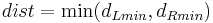 . Therefore for each point
  of the left of the dividing line we have to compare the distances to the points that lie in the rectangle of dimensions (dist, 2 * dist) to the right of the dividing line, as shown in the figure. And what is more, this rectangle can contain at most 6 points with pairwise distances at most . Therefore it is sufficient to compute at most 8(n) left-right distances in step 4. The recurrence relation for the number of steps can be written as
 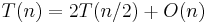 , which we can solve using the master theorem to get O(n log n).
As the closest pair of points define an edge in the Delaunay triangulation, and correspond to two adjacent cells in the Voronoi diagram, the closest pair of points can be determined in linear time when we are given one of these two structures. Computing either the Delaunay triangulation or the Voronoi diagram takes O(n log n) time. These approaches are not efficient for dimension d>2, while the divide and conquer algorithm can be generalized to take O(n log n) time for any constant value of d.
Dynamic closest-pair problem
The dynamic version for the closest-pair problem is stated as follows:
- Given a dynamic set of objects, find algorithms and data structures for efficient recalculation of the closest pair of objects each time the objects are inserted or deleted.
If the bounding box for all points is known in advance and the constant-time floor function is available, then the expected O(n) space data structure was suggested that supports expected-time O(log n) insertions and deletions and constant query time. When modified for the algebraic decision tree model, insertions and deletions would require O(log2 n) expected time. [5] It is worth noting, though, that the complexity of the dynamic closest pair algorithm cited above is exponential in the dimension d, and therefore such an algorithm becomes less suitable for high-dimensional problems.
Notes
- ^ a b M. I. Shamos and D. Hoey. "Closest-point problems." In Proc. 16th Annual IEEE Symposium on Foundations of Computer Science (FOCS), pp. 151—162, 1975
- ^ S. Fortune and J.E. Hopcroft. "A note on Rabin's nearest-neighbor algorithm." Information Processing Letters, 8(1), pp. 20—23, 1979
- ^ S. Khuller and Y. Matias. A simple randomized sieve algorithm for the closest-pair problem. Inf. Comput., 118(1):34—37,1995
- ^ Richard Lipton (24 September 2011). "Rabin Flips a Coin". http://rjlipton.wordpress.com/2009/03/01/rabin-flips-a-coin/.
- ^ Mordecai Golin, Rajeev Raman, Christian Schwarz, Michiel Smid, "Randomized Data Structures For The Dynamic Closest-Pair Problem", SIAM J. Comput., vo. 26, no. 4, 1998, preliminary version reported at the 4th Annu. ACM-SIAM Symp. on Discrete Algorithms, pp. 301–310 (1993)
References
- Thomas H. Cormen, Charles E. Leiserson, Ronald L. Rivest, and Clifford Stein. Introduction to Algorithms, Second Edition. MIT Press and McGraw-Hill, 2001. ISBN 0-262-03293-7. Pages 957–961 of section 33.4: Finding the closest pair of points.
- Jon Kleinberg; Éva Tardos (2006). Algorithm Design. Addison Wesley.
- UCSB Lecture Notes
- rosettacode.org - Closest pair of points implemented in multiple programming languages
- Line sweep algorithm for the closest pair problem