Betweenness centrality

Betweenness centrality is a measure of a node's centrality in a network equal to the number of shortest paths from all vertices to all others that pass through that node. Betweenness centrality is a more useful measure of the load placed on the given node in the network as well as the node's importance to the network than just connectivity. The latter is only a local effect while the former is more global to the network. Development of betweenness centrality is generally attributed to sociologist Linton Freeman, who has also developed a number of other centrality measures.^[1] (The same idea was also earlier proposed by mathematician J. Anthonisse, but his work was never published.^[1])

1 Definition
2 The load distribution in real and model networks
- 2.1 Model networks
- 2.2 Real networks
3 Weighted networks
4 Algorithms
5 See also
6 References

Definition

The betweenness centrality of a node $v$ is given by the expression:

$g(v)= \sum_{s \neq v \neq t}\frac{\sigma_{st}(v)}{\sigma_{st}}$

where $\sigma_{st}$ total number of shortest paths from node $s$ to node $t$ and $\sigma_{st}(v)$ is the number of those paths that pass through $v$ .

Note that the betweenness centrality of a node scales with the number of pairs of nodes as implied by the summation indices. Therefore the calculation may be rescaled by dividing through by the number of pairs of nodes not including $v$ , so that $g \in [0,1]$ . The division is done by $(N-1)(N-2)$ for directed graphs and $(N-1)(N-2)/2$ for undirected graphs, where $N$ is the number of nodes in the giant component. Note that this scales for the highest possible value, where one node is crossed by every single shortest path. This is often not the case, and a normalization can be performed without a loss of precision

$normal(g(v)) = \frac{g(v) - min(g)}{max(g) - max(g)}$

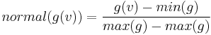
which results in:

$max(normal) = 1$

$min(normal) = 0$

Note that this will always be a scaling from a smaller range into a larger range, so no precision is lost.

The load distribution in real and model networks

Model networks

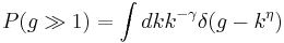
It has been shown that the load distribution of a scale free network follows a power law given by a load exponent $\delta$ ,^[2]

$P(g) \approx g^{-\delta}$ (1)

this implies the scaling relation to the degree of the node,

$g(k) \approx k^\eta$ .

Where $g(k)$ is the average load of vertices with degree $k$ . The exponents $\delta$ and $\eta$ are not independent since equation (1) implies ^[3]

$P(g)= \int dk P(k) \delta (g-k^\eta)$

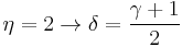
For large g , and therefore large k , the expression becomes

$P(g\gg1)= \int dk k^{-\gamma} \delta (g-k^\eta)$

$\sim g^{-1-\frac{\gamma -1}{\eta}}$

which proves the following equality:

$\eta=\frac{\gamma -1}{\delta -1}$

The important exponent appears to be $\eta$ which describes how the betweenness centrality depends on the connectivity. The situation which maximizes the betweenness centrality for a vertex is when all shortest paths are going through it, which corresponds to a tree structure (a network with no clustering). In the case of a tree network the maximum value of $\eta = 2$ is reached.^[3]

$\eta = 2 \rarr \delta = \frac{\gamma %2B1}{2}$

This maximal value of $\eta$ (and hence minimum of $\delta$ ) puts bounds on the load exponents for networks with non-vanishing clustering.

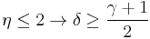
$\eta \le 2 \rarr \delta \ge \frac{\gamma %2B1}{2}$

In this case, the exponents $\delta , \eta$ are not universal and depend on the different details (average connectivity, correlations, etc.)

Real networks

Real world scale free networks, such as the internet, also follow a power law load distribution.^[4] This is an intuitive result. Scale free networks arrange themselves to create short path lengths across the network by creating a few hub nodes with much higher connectivity than the majority of the network. These hubs will naturally experience much higher loads because of this added connectivity.

Weighted networks

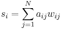
In a weighted network the links connecting the nodes are no longer treated as binary interactions, but are weighted in proportion to their capacity, influence, frequency, etc., which adds another dimension of heterogeneity within the network beyond the topological effects. A node's strength in a weighted network is given by its degree multiplied by the sum of its link's weights,

$s_{i} = \sum_{j=1}^{N} a_{ij}w_{ij}$

With $a_{ij}$ and $w_{ij}$ being adjacency and weight matricies between nodes $i$ and $j$ , respectively. Analogous to the power law distribution of degree found in scale free networks, the strength of a given node follows a power law distribution as well.

$s(k) \approx k^\beta \,$

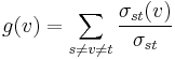
A study of the average value $s(b)$ of the strength for vertices with betweenness $b$ shows that the functional behavior can be approximated by a scaling form ^[5]

$s(b)\approx b^{\alpha}$

Algorithms

Calculating the betweenness and closeness centralities of all the vertices in a graph involves calculating the shortest paths between all pairs of vertices on a graph. This takes $\Theta(V^3)$ time with the Floyd–Warshall algorithm, modified to not only find one but count all shortest paths between two nodes. On a sparse graph, Johnson's algorithm may be more efficient, taking $O(V^2 \log V %2B V E)$ time. On unweighted graphs, calculating betweenness centrality takes $O(V E)$ time using Brandes' algorithm.^[6]

In calculating betweenness and closeness centralities of all vertices in a graph, it is assumed that graphs are undirected and connected with the allowance of loops and multiple edges. When specifically dealing with network graphs, oftentimes graphs are without loops or multiple edges to maintain simple relationships (where edges represent connections between two people or vertices). In this case, using Brandes' algorithm will divide final centrality scores by 2 to account for each shortest path being counted twice.^[6]

References

^ ^a ^b Newman, M.E.J. 2010. Networks: An Introduction. Oxford, UK: Oxford University Press.
^ ^a ^b K.-I. Goh, B. Kahng, and D. Kim PhysRevLett.87.278701
^ ^a ^b M. Barthélemy Eur. Phys. J. B 38, 163–168 (2004)
^ Kwang-Il Goh, Eulsik Oh, Hawoong Jeong, Byungnam Kahng, and Doochul Kim. PNAS (2002) vol. 99 no. 2
^ A. Barrat, M. Barthelemy, R. Pastor-Satorras, and A. Vespignani. PNAS (2004) vol. 101 no. 11
^ ^a ^b Ulrik Brandes (PDF). A faster algorithm for betweenness centrality. http://www.cs.ucc.ie/~rb4/resources/Brandes.pdf.