Baker–Campbell–Hausdorff formula

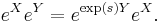
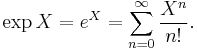
In mathematics, the Baker–Campbell–Hausdorff formula is the solution to

$Z = \log(e^X e^Y)\,$

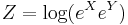
for noncommutative X and Y. This formula links Lie groups to Lie algebras by expressing the logarithm of the product of two Lie group elements as a Lie algebra element in canonical coordinates, a significant guiding connection appreciated (Hausdorff 1906)^[1] before the full development of the theory.

It is named for Henry Frederick Baker, John Edward Campbell, and Felix Hausdorff. It was first noted in print by Campbell^[2] (1897); elaborated by Henri Poincaré^[3] (1899) and Baker (1902);^[4] and systematized geometrically, and linked to the Jacobi identity by Hausdorff (1906).^[1]

1 The Baker–Campbell–Hausdorff formula: existence
2 An explicit Baker–Campbell–Hausdorff formula
- 2.1 Selected tractable cases
- 2.2 Matrix Lie group illustration
3 The Zassenhaus formula
4 The Hadamard lemma
5 Application in Quantum Mechanics
6 See also
7 References
8 Bibliography
9 External links

The Baker–Campbell–Hausdorff formula: existence

The Baker–Campbell–Hausdorff formula implies that if X and Y are in some Lie algebra $\mathfrak g,$ defined over any field of characteristic 0, then

log(exp(X) exp(Y)),

can be written as a formal infinite sum of elements of $\mathfrak g$ . For many applications, one does not need an explicit expression for this infinite sum, but merely assurance of its existence, and this can be seen as follows. The ring

S = R[[X,Y]]

of all non-commuting formal power series in non-commuting variables X and Y has a ring homomorphism Δ from S to the completion of

S⊗S,

called the coproduct, such that

Δ(X) = X⊗1 + 1⊗X

and similarly for Y. (The definition of the coproduct is extended recursively by the rule $\Delta(XY) = \Delta(X)\Delta(Y)$ ). This has the following properties:

exp is an isomorphism (of sets) from the elements of S with constant term 0 to the elements with constant term 1, with inverse log
r=exp(s) is grouplike (this means Δ(r)=r⊗r) if and only if s is primitive (this means Δ(s)=s⊗1+1⊗s).
The grouplike elements form a group under multiplication.
The primitive elements are exactly the formal infinite sums of elements of the Lie algebra generated by X and Y. (Friedrichs' theorem ^[5])

The existence of the Baker–Campbell–Hausdorff formula can now be seen as follows: The elements X and Y are primitive, so exp(X) and exp(Y) are grouplike, so their product exp(X)exp(Y) is also grouplike, so its logarithm log(exp(X)exp(Y)) is primitive, and hence can be written as an infinite sum of elements of the Lie algebra generated by X and Y.

The universal enveloping algebra of the free Lie algebra generated by X and Y is isomorphic to the algebra of all non-commuting polynomials in X and Y. In common with all universal enveloping algebras, it has a natural structure of a Hopf algebra, with a coproduct Δ. The ring S used above is just a completion of this Hopf algebra.

An explicit Baker–Campbell–Hausdorff formula

Specifically, let G be a simply-connected Lie group with Lie algebra $\mathfrak g$ . Let

$\exp�: \mathfrak g\rightarrow G$

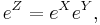
be the exponential map. The following general combinatoric formula was introduced by Eugene Dynkin (1947):^[6]

$\log(\exp X\exp Y) = \sum_{n>0}\frac {(-1)^{n-1}}{n} \sum_{ \begin{smallmatrix} {r_i %2B s_i > 0} \\ {1\le i \le n} \end{smallmatrix}} \frac{(\sum_{i=1}^n (r_i%2Bs_i))^{-1}}{r_1!s_1!\cdots r_n!s_n!} [ X^{r_1} Y^{s_1} X^{r_2} Y^{s_2} \ldots X^{r_n} Y^{s_n} ],$

which uses the notation

$[ X^{r_1} Y^{s_1} \ldots X^{r_n} Y^{s_n} ] = [ \underbrace{X,[X,\ldots[X}_{r_1} ,[ \underbrace{Y,[Y,\ldots[Y}_{s_1} ,\,\ldots\, [ \underbrace{X,[X,\ldots[X}_{r_n} ,[ \underbrace{Y,[Y,\ldots Y}_{s_n} ]]\ldots]].$

This term is zero if $s_n > 1$ or if $s_n = 0$ and $r_n > 1$ .^[7]

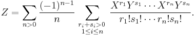
The first few terms are well-known, with all higher-order terms involving [X,Y] and commutator nestings thereof (thus in the Lie algebra):

$\begin{align} Z(X,Y)&{}=\log(\exp X\exp Y) \\ &{}= X %2B Y %2B \frac{1}{2}[X,Y] %2B \frac{1}{12}[X,[X,Y]] - \frac{1}{12}[Y,[X,Y]] \\ &{}\quad - \frac {1}{24}[Y,[X,[X,Y]]] \\ &{}\quad - \frac{1}{720}([[[[X,Y],Y],Y],Y] %2B[[[[Y,X],X],X],X]) \\ &{}\quad %2B\frac{1}{360}([[[[X,Y],Y],Y],X]%2B[[[[Y,X],X],X],Y])\\ &{}\quad %2B \frac{1}{120}([[[[Y,X],Y],X],Y] %2B[[[[X,Y],X],Y],X]) %2B \cdots \end{align}$

Note the X-Y (anti-)/symmetry in alternating orders of the expansion, since Z(Y, X) = −Z(−X, −Y).

Selected tractable cases

There is no expression in closed form for an arbitrary Lie algebra, though there are exceptional tractable cases, as well as efficient algorithms for working out the expansion in applications.

For example, if [X, Y] vanishes, then the above formula reduces to X + Y. If the commutator [X, Y] is a scalar (central), then all but the first three terms on the right-hand side of the above vanish. (This is the degenerate case utilized in quantum mechanics, as illustrated below.)

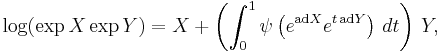
Other forms of the Campbell–Baker–Hausdorff formula, emphasizing expansion in terms of the element Y (and using the linear Adjoint endomorphism notation, adX Y ≡ [X,Y]), might serve well:

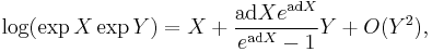
$\log(\exp X\exp Y) = X %2B \frac{\text{ad} X e^{\text{ad} X}}{e^{\text{ad} X}-1} Y %2B O(Y^2),$

as is evident from the integral formula below. (The coefficients of the nested commutators linear in Y are normalized Bernoulli numbers, outlined below.) Thus, when the commutator happens to be [X, Y] = sY, for some non-zero s, this formula reduces to just Z = X + sY / (1 − exp(−s)), which then leads to braiding identities such as

$e^{X} e^{Y} = e^{\exp (s) Y} e^{X}.\,$

There are numerous such well-known expressions applied routinely in physics.^[8] A popular integral formula is^[9]

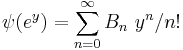
$\log(\exp X\exp Y) = X %2B \left ( \int^1_0 \psi \left ( e^{\text{ad} X} e^{t \,\text{ad} Y}\right ) \, dt \right) \, Y,$

involving a generating function for the Bernoulli numbers,

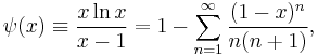
$\psi(x) \equiv \frac{x \ln x}{x-1}= 1- \sum^\infty_{n=1} {(1-x)^n \over n (n%2B1)},$

utilized by Poincaré and Hausdorff. Recall

$\psi(e^y)=\sum_{n=0}^\infty B_n ~ y^n/n!$ ,

for the Bernoulli numbers, B₀ = 1 , B₁ = 1/2 , B₂ = 1/6 , B₄ = -1/30 , ...

Matrix Lie group illustration

For a matrix Lie group 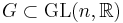$G \sub \mbox{GL}(n,\mathbb{R})$ the Lie algebra is the tangent space of the identity I, and the commutator is simply [X, Y] = XY − YX; the exponential map is the standard exponential map of matrices,

$\exp X = e^X = \sum_{n=0}^{\infty}{\frac{X^n}{n!}}.$

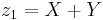
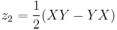
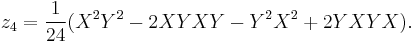
When one solves for Z in

$e^Z = e^X e^Y,\,\!$

one obtains a simpler formula:

$Z = \sum_{n>0} \frac{(-1)^{n-1}}{n} \sum_{\begin{smallmatrix} r_i%2Bs_i>0\, \\ 1\le i\le n\end{smallmatrix}} \frac{X^{r_1}Y^{s_1}\cdots X^{r_n}Y^{s_n}}{r_1!s_1!\cdots r_n!s_n!}.$

The first, second, third, and fourth order terms are:

$z_1 = X %2B Y\,\!$

$z_2 = \frac{1}{2} (XY - YX)$

$z_3 = \frac{1}{12} (X^2Y %2B XY^2 - 2XYX %2B Y^2X %2B YX^2 - 2YXY)$

$z_4 = \frac{1}{24} (X^2Y^2 - 2XYXY - Y^2X^2 %2B 2YXYX).$

The Zassenhaus formula

A related combinatoric expansion that is useful in dual^[8] applications is

$e^{t(X%2BY)}= e^{tX}~ e^{tY} ~e^{-\frac{t^2}{2} [X,Y]} ~ e^{\frac{t^3}{6}(2[Y,[X,Y]]%2B [X,[X,Y]] )} ~ e^{\frac{-t^4}{24}([[[X,Y],X],X] %2B 3[[[X,Y],X],Y] %2B 3[[[X,Y],Y],Y]) } \cdots$

where exponents of higher order in t are likewise nested commutators.

The Hadamard lemma

Let $L_n$ be the space of all complex $n \times n$ matrices, and let $\operatorname{ad}\,X$ be the linear operator defined by $\operatorname{ad}\,X = [X, Y]$ for some fixed $Y \in L_n$ . A standard combinatorial lemma that is utilized^[9] in the above explicit expansions is

$e^{X}Y e^{-X} = e^{\operatorname{ad}\,X} Y =Y%2B\left[X,Y\right]%2B\frac{1}{2!}[X,[X,Y]]%2B\frac{1}{3!}[X,[X,[X,Y]]]%2B\cdots.$

This formula can be proved by parametric induction: evaluation of the derivative with respect to s of f (s)≡ $e^{sX}Y e^{-sX}$ ; recursive determination of the Taylor expansion coefficients around s=0, in terms of nested commutators; and evaluation at s =1, namely f (1).

Application in Quantum Mechanics

A degenerate form of the Campbell–Baker–Hausdorff formula is useful in Quantum Mechanics, where X and Y are Hilbert space operators.

A typical example is the annihilation and creation operators, $\hat{a}$ and $\hat{a}^{\dagger}$ . Their commutator $[\hat{a}, \hat{a}^{\dagger}]$ is central: it commutes with both $\hat{a}$ and $\hat{a}^{\dagger}$ . As indicated above, the expansion then collapses to the semi-trivial degenerate form:

$e^{v\hat{a}^{\dagger} - v^*\hat{a}} = e^{v\hat{a}^{\dagger}} e^{-v^*\hat{a}} e^{-|v|^{2}/2} ,$

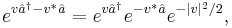
where $v$ is a mere complex number.

This example illustrates the resolution of the displacement operator, $e^{v\hat{a}^{\dagger} - v^*\hat{a}}$ into exponentials of the annihilation operator, creation operator and c-numbers.^[10] This degenerate Campbell–Baker–Hausdorff formula displays the product of two displacement operators as another displacement operator (up to a phase factor), with the resultant displacement equal to the sum of the two displacements, viz. the Heisenberg group:

$e^{v\hat{a}^{\dagger} - v^*\hat{a}} e^{u\hat{a}^{\dagger} - u^*\hat{a}} = e^{(v%2Bu)\hat{a}^{\dagger} - (v^*%2Bu^*)\hat{a}} e^{(vu^*-uv^*)/2}.$

References

^ ^a ^b F. Hausdorff, "Die symbolische Exponentialformel in der Gruppentheorie", Ber Verh Saechs Akad Wiss Leipzig 58 (1906) 19–48.
^ J. Campbell, Proc Lond Math Soc 28 (1897) 381–390; ibid 29 (1898) 14–32.
^ H. Poincaré, Compt Rend Acad Sci Paris 128 (1899) 1065–1069; Camb Philos Trans 18 (1899) 220–255.
^ H. Baker, Proc Lond Math Soc (1) 34 (1902) 347–360; ibid (1) 35 (1903) 333–374; ibid (Ser 2) 3 (1905) 24–47.
^ N. Jacobson, Lie Algebras, John Wiley & Sons, 1966.
^ Dynkin, Eugene Borisovich (1947). "[Calculation of the coefficients in the Campbell–Hausdorff formula]". Doklady Akademii Nauk SSSR 57: 323–326.
^ A.A. Sagle & R.E. Walde, "Introduction to Lie Groups and Lie Algebras", Academic Press, New York, 1973. ISBN 0-12-614550-4.
^ ^a ^b W. Magnus, Comm Pur Appl Math VII (1954) 649–673.
^ ^a ^b W. Miller, Symmetry Groups and their Applications, Academic Press, New York, 1972, pp 159–161. ISBN 0-12-497460-0
^ L. Mandel, E. Wolf Optical Coherence and Quantum Optics (Cambridge 1995).

Bibliography

Yu.A. Bakhturin (2001), "Campbell–Hausdorff formula", in Hazewinkel, Michiel, Encyclopedia of Mathematics, Springer, ISBN 978-1556080104, http://www.encyclopediaofmath.org/index.php?title=C/c020090
L. Corwin & F.P Greenleaf, Representation of nilpotent Lie groups and their applications, Part 1: Basic theory and examples, Cambridge University Press, New York, 1990, ISBN 0-521-36034-X.
Brian C. Hall, Lie Groups, Lie Algebras, and Representations: An Elementary Introduction, Springer, 2003. ISBN 0-387-40122-9
H. Kleinert, Path Integrals in Quantum Mechanics, Statistics, Polymer Physics, and Financial Markets, World Scientific (Singapore, 2006).
M.W. Reinsch, "A simple expression for the terms in the Baker–Campbell–Hausdorff series". Jou Math Phys, 41(4):2434–2442, (2000). doi:10.1063/1.533250
W. Rossmann, Lie Groups: An Introduction through Linear Groups. Oxford University Press, 2002.
J.-P. Serre, Lie algebras and Lie groups , Benjamin, 1965.