Triangular matrix

A related concept is that of a triangular array.

For the rings, see triangular matrix ring.

In the mathematical discipline of linear algebra, a triangular matrix is a special kind of square matrix where either all the entries below or all the entries above the main diagonal are zero. A matrix which is similar to a triangular matrix is called triangularizable.

Because matrix equations with triangular matrices are easier to solve they are very important in numerical analysis. The LU decomposition gives an algorithm to decompose any invertible matrix A into two triangular factors: a normed lower triangle matrix L and an upper triangle matrix U.

1 Description
2 Special forms
3 Special properties
4 Triangularisability
- 4.1 Simultaneous triangularisability
5 Generalizations
- 5.1 Borel subgroups and Borel subalgebras
- 5.2 Examples
6 Examples
7 Forward and back substitution
8 See also
9 Notes
10 References

Description

A matrix of the form

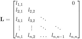
$\mathbf{L}= \begin{bmatrix} l_{1,1} & & & & 0 \\ l_{2,1} & l_{2,2} & & & \\ l_{3,1} & l_{3,2} & \ddots & & \\ \vdots & \vdots & \ddots & \ddots & \\ l_{n,1} & l_{n,2} & \ldots & l_{n,n-1} & l_{n,n} \end{bmatrix}$

is called lower triangular matrix or left triangular matrix, and analogously a matrix of the form

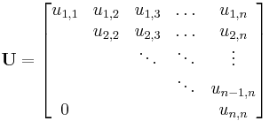
$\mathbf{U} = \begin{bmatrix} u_{1,1} & u_{1,2} & u_{1,3} & \ldots & u_{1,n} \\ & u_{2,2} & u_{2,3} & \ldots & u_{2,n} \\ & & \ddots & \ddots & \vdots \\ & & & \ddots & u_{n-1,n}\\ 0 & & & & u_{n,n} \end{bmatrix}$

is called upper triangular matrix or right triangular matrix.

The standard operations on triangular matrices conveniently preserve the triangular form: the sum and product of two upper triangular matrices is again upper triangular. The inverse of an upper triangular matrix is also upper triangular, and of course we can multiply an upper triangular matrix by a constant and it will still be upper triangular. This means that the upper triangular matrices form a subalgebra of the ring of square matrices for any given size. The analogous result holds for lower triangular matrices. Note, however, that the product of a lower triangular with an upper triangular matrix does not preserve triangularity.

Special forms

Strictly triangular matrix

A triangular matrix with zero entries on the main diagonal is strictly upper or lower triangular. All strictly triangular matrices are nilpotent, and they form a nilpotent Lie algebra, denoted $\mathfrak{n}.$ Strictly upper triangular matrices are the derived Lie algebra of the Lie algebra $\mathfrak{b}$ of all upper triangular matrices; symbolically, $\mathfrak{n} = [\mathfrak{b},\mathfrak{b}].$ Strictly upper triangular matrices are the Lie algebra of the Lie group of unitriangular matrices.

In fact, by Engel's theorem, any nilpotent Lie algebra is conjugate to a subalgebra of the strictly upper triangular matrices: a nilpotent Lie algebra is simultaneously strictly upper triangularizable.

Unitriangular matrix

If the entries on the main diagonal are 1, the matrix is called (upper or lower) unitriangular. All unitriangular matrices are unipotent. Other names used for these matrices are unit (upper or lower) triangular (of which "unitriangular" might be a contraction), or normed upper/lower triangular (very rarely used). However a unit triangular matrix is not the same as the unit matrix, and a normed triangular matrix has nothing to do with the notion of matrix norm.

Unitriangular matrices form a Lie group, whose Lie algebra is the strictly upper triangular matrices.

Gauss matrix

A Gauss matrix is a special form of a unitriangular matrix, where all of the off-diagonal entries are zero, except for the entries in one column. Such a matrix is also called atomic upper/lower triangular or Gauss transformation matrix. So an atomic lower triangular matrix is of the form

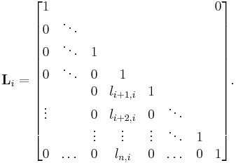
$\mathbf{L}_{i} = \begin{bmatrix} 1 & & & & & & & 0 \\ 0 & \ddots & & & & & & \\ 0 & \ddots & 1 & & & & & \\ 0 & \ddots & 0 & 1 & & & & \\ & & 0 & l_{i%2B1,i} & 1 & & & \\ \vdots & & 0 & l_{i%2B2,i} & 0 & \ddots & & \\ & & \vdots & \vdots & \vdots & \ddots & 1 & \\ 0 & \dots & 0 & l_{n,i} & 0 & \dots & 0 & 1 \\ \end{bmatrix}.$

The inverse of an atomic triangular matrix is again atomic triangular. Indeed, we have

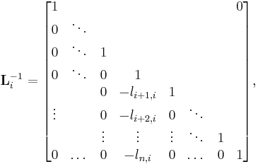
$\mathbf{L}_{i}^{-1} = \begin{bmatrix} 1 & & & & & & & 0 \\ 0 & \ddots & & & & & & \\ 0 & \ddots & 1 & & & & & \\ 0 & \ddots & 0 & 1 & & & & \\ & & 0 & -l_{i%2B1,i} & 1 & & & \\ \vdots & & 0 & -l_{i%2B2,i} & 0 & \ddots & & \\ & & \vdots & \vdots & \vdots & \ddots & 1 & \\ 0 & \dots & 0 & -l_{n,i} & 0 & \dots & 0 & 1 \\ \end{bmatrix},$

i.e., the single column of off-diagonal entries are replaced in the inverse matrix by their additive inverses.

Special properties

A matrix which is simultaneously upper and lower triangular is diagonal. The identity matrix is the only matrix which is both upper and lower unitriangular.

A matrix which is simultaneously triangular and normal is also diagonal. This can be seen by looking at the diagonal entries of A^*A and AA^*, where A is a normal, triangular matrix.

The transpose of an upper triangular matrix is a lower triangular matrix and vice versa.

The determinant of a triangular matrix equals the product of the diagonal entries. Since for any triangular matrix A the matrix $x I-A$ , whose determinant is the characteristic polynomial of A, is also triangular, the diagonal entries of A in fact give the multiset of eigenvalues of A (an eigenvalue with multiplicity m occurs exactly m times as diagonal entry).^[1]

The variable L is commonly used for lower triangular matrix, standing for lower/left, while the variable U or R is commonly used for upper triangular matrix, standing for upper/right.

Many operations can be performed more easily on triangular matrices than on general matrices. Notably matrix inversion (when possible) can be done by back substitution, avoiding the complications of general Gaussian elimination.

The inverse of a triangular matrix is also triangular.

The product of two lower triangular matrices produces a lower triangular matrix.

The product of two upper triangular matrices produces an upper triangular matrix.

Triangularisability

A matrix that is similar to a triangular matrix is referred to as triangularisable. Abstractly, this is equivalent to stabilising a flag: upper triangular matrices are precisely those that preserve the standard flag, which is given by the standard ordered basis $(e_1,\ldots,e_n)$ and the resulting flag $0 < \left\langle e_1\right\rangle < \left\langle e_1,e_2\right\rangle < \cdots < \left\langle e_1,\ldots,e_n \right\rangle = K^n.$ All flags are conjugate (as the general linear group acts transitively on bases), so any matrix that stabilises a flag is similar to one that stabilises the standard flag.

Any complex square matrix is triangularisable.^[1] In fact, a matrix A over a field containing all of the eigenvalues of A (for example, any matrix over an algebraically closed field) is similar to a triangular matrix. This can be proven by using induction on the fact that A has an eigenvector, by taking the quotient space by the eigenvector and inducting to show that A stabilises a flag, and is thus triangularisable with respect to a basis for that flag.

A more precise statement is given by the Jordan normal form theorem, which states that in this situation, A is similar to an upper triangular matrix of a very particular form. The simpler triangularization result is often sufficient however, and in any case used in proving the Jordan normal form theorem.^[1]^[2]

In the case of complex matrices, it is possible to say more about triangularisation, namely, that any square matrix A has a Schur decomposition. This means that A is unitarily equivalent (i.e. similar, using a unitary matrix as change of basis) to an upper triangular matrix; this follows by taking an Hermitian basis for the flag.

Simultaneous triangularisability

Generalizations

Because the product of two upper triangular matrices is again upper triangular, the set of upper triangular matrices forms an algebra. Algebras of upper triangular matrices have a natural generalization in functional analysis which yields nest algebras on Hilbert spaces.

A non-square (or sometimes any) matrix with zeros above (below) the diagonal is called a lower (upper) trapezoidal matrix. The non-zero entries form the shape of a trapezoid.

Borel subgroups and Borel subalgebras

Main articles: Borel subgroup and Borel subalgebra

The set of invertible triangular matrices of a given kind (upper or lower) forms a group, indeed a Lie group, which is a subgroup of the general linear group of all invertible matrices; invertible is equivalent to all diagonal entries being invertible (non-zero).

Over the real numbers, this group is disconnected, having $2^n$ components accordingly as each diagonal entry is positive or negative. The identity component is invertible triangular matrices with positive entries on the diagonal, and the group of all invertible triangular matrices is a semidirect product of this group and diagonal entries with $\pm 1$ on the diagonal, corresponding to the components.

The Lie algebra of the Lie group of invertible upper triangular matrices is the set of all upper triangular matrices, not necessarily invertible, and is a solvable Lie algebra. These are, respectively, the standard Borel subgroup B of the Lie group GL_n and the standard Borel subalgebra $\mathfrak{b}$ of the Lie algebra gl_n.

The upper triangular matrices are precisely those that stabilize the standard flag. The invertible ones among them form a subgroup of the general linear group, whose conjugate subgroups are those defined as the stabilizer of some (other) complete flag. These subgroups are Borel subgroups. The group of invertible lower triangular matrices is such a subgroup, since it is the stabilizer of the standard flag associated to the standard basis in reverse order.

The stabilizer of a partial flag obtained by forgetting some parts of the standard flag can be described as a set of block upper triangular matrices (but its elements are not all triangular matrices). The conjugates of such a group are the subgroups defined as the stabilizer of some partial flag. These subgroups are called parabolic subgroups.

Examples

The group of 2 by 2 upper unitriangular matrices is isomorphic to the additive group of the field of scalars; in the case of complex numbers it corresponds to a group formed of parabolic Möbius transformations; the 3 by 3 upper unitriangular matrices form the Heisenberg group.

Examples

The matrix

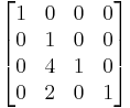
$\begin{bmatrix} 1 & 4 & 2 \\ 0 & 3 & 4 \\ 0 & 0 & 1 \\ \end{bmatrix}$

is upper triangular and

$\begin{bmatrix} 1 & 0 & 0 \\ 2 & 8 & 0 \\ 4 & 9 & 7 \\ \end{bmatrix}$

is lower triangular.

The matrix

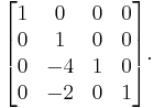
$\begin{bmatrix} 1 & 0 & 0 & 0 \\ 0 & 1 & 0 & 0 \\ 0 & 4 & 1 & 0 \\ 0 & 2 & 0 & 1 \\ \end{bmatrix}$

is atomic lower triangular. Its inverse is

$\begin{bmatrix} 1 & 0 & 0 & 0 \\ 0 & 1 & 0 & 0 \\ 0 & -4 & 1 & 0 \\ 0 & -2 & 0 & 1 \\ \end{bmatrix}.$

Forward and back substitution

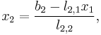
A matrix equation in the form $\mathbf{L}\mathbf{x} = \mathbf{b}$ or $\mathbf{U} \mathbf{x} = \mathbf{b}$ is very easy to solve by an iterative process called forward substitution for lower triangular matrices and analogously back substitution for upper triangular matrices. The process is so called because for lower triangular matrices, one first computes $x_1$ , then substitutes that forward into the next equation to solve for $x_2$ , and repeats through to $x_n$ . In an upper triangular matrix, one works backwards, first computing $x_n$ , then substituting that back into the previous equation to solve for $x_{n-1}$ , and repeating through $x_1$ .

Notice that this does not require inverting the matrix.

Forward substitution

The matrix equation Lx = b can be written as a system of linear equations

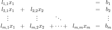
$\begin{matrix} l_{1,1} x_1 & & & & & = & b_1 \\ l_{2,1} x_1 & %2B & l_{2,2} x_2 & & & = & b_2 \\ \vdots & & \vdots & \ddots & & & \vdots \\ l_{m,1} x_1 & %2B & l_{m,2} x_2 & %2B \dotsb %2B & l_{m,m} x_m & = & b_m \\ \end{matrix}$

Observe that the first equation ( $l_{1,1} x_1 = b_1$ ) only involves $x_1$ , and thus one can solve for $x_1$ directly. The second equation only involves $x_1$ and $x_2$ , and thus can be solved once one substitutes in the already solved value for $x_1$ . Continuing in this way, the $k$ -th equation only involves $x_1,\dots,x_k$ , and one can solve for $x_k$ using the previously solved values for $x_1,\dots,x_{k-1}$ .

The resulting formulas are:

$x_1 = \frac{b_1}{l_{1,1}},$

$x_2 = \frac{b_2 - l_{2,1} x_1}{l_{2,2}},$

$\vdots$

$x_m = \frac{b_m - \sum_{i=1}^{m-1} l_{m,i}x_i}{l_{m,m}}.$

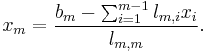
A matrix equation with an upper triangular matrix U can be solved in an analogous way, only working backwards.

Algorithm

The following is an example implementation of this algorithm in the C# programming language. Note that the algorithm performs poorly in C# due to the inefficient handling of non-jagged matrices in this language. Nonetheless, the method of forward and backward substitution can be highly efficient.

 double[] luEvaluate(double[,] L, double[,] U, Vector b)
  {
  // Ax = b -> LUx = b. Then y is defined to be Ux
  int i = 0;
  int j = 0;
  int n = b.Count;
  double[] x = new double[n];
  double[] y = new double[n];
  // Forward solve Ly = b
  for (i = 0; i < n; i++)
  {
    y[i] = b[i];
    for (j = 0; j < i; j++)
    {
      y[i] -= L[i, j] * y[j];
    }
    y[i] /= L[i, i];
  }
  // Backward solve Ux = y
  for (i = n - 1; i >= 0; i--)
  {
    x[i] = y[i];
    for (j = i + 1; j < n; j++)
    {
      x[i] -= U[i, j] * x[j];
    }
    x[i] /= U[i, i];
  }
  return x;
 }

Applications

Forward substitution is used in financial bootstrapping to construct a yield curve.

Notes

References

^ ^a ^b ^c (Axler 1996, pp. 86–87, 169)
^ (Herstein 1975, pp. 285–290)

Axler, Sheldon (1996), Linear Algebra Done Right, Springer-Verlag, ISBN 0-387-98258-2
Drazin, M. P.; Dungey, J. W.; Gruenberg, K. W. (1951), "Some theorems on commutative matrices", J. London Math. Soc. 26: 221–228, http://jlms.oxfordjournals.org/cgi/pdf_extract/s1-26/3/221
Herstein, I. N. (1975), Topics in Algebra (2nd edition ed.), John Wiley and Sons, ISBN 0-471-01090-1
Prasolov, Viktor (1994), Problems and theorems in linear algebra, http://books.google.com/books?id=fuONq1od6nsC&lpg=PP1&dq=victor%20prasolov%20Problems%20and%20theorems%20in%20linear%20algebra&pg=PP1#v=onepage&q&f=false

Numerical linear algebra

Key concepts	Floating point · Numerical stability · BLAS

Problems	Matrix multiplication · Matrix decompositions · Linear equations · Sparse problems

Hardware	CPU cache · TLB · Cache-oblivious algorithm · SIMD · Multiprocessing

Software	Specialized libraries · General purpose software

Triangular matrix

Contents

Description

Special forms

Strictly triangular matrix

Unitriangular matrix

Gauss matrix

Special properties

Triangularisability

Simultaneous triangularisability

Generalizations

Borel subgroups and Borel subalgebras

Examples

Examples

Forward and back substitution

Forward substitution

Algorithm

Applications

See also

Notes

References