Gauss–Markov theorem

Not to be confused with Gauss–Markov process.

In statistics, the Gauss–Markov theorem, named after Carl Friedrich Gauss and Andrey Markov, states that in a linear regression model in which the errors have expectation zero and are uncorrelated and have equal variances, the best linear unbiased estimator (BLUE) of the coefficients is given by the ordinary least squares estimator. Here "best" means giving the lowest possible mean squared error of the estimate. The errors need not be normal, nor independent and identically distributed (only uncorrelated and homoscedastic).

1 Statement
2 Proof
3 Generalized least squares estimator
4 See also
- 4.1 Other unbiased statistics
5 Notes
6 References
7 External links

Statement

Suppose we have

$Y_i=\sum_{j=1}^{K}\beta_j X_{ij}%2B\varepsilon_i$

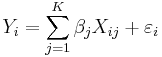
for i = 1, . . ., n, where β_j are non-random but unobservable parameters, X_ij are non-random and observable (called the "explanatory variables"), ε_i are random, and so Y_i are random. The random variables ε_i are called the "errors" (not to be confused with "residuals"; see errors and residuals in statistics). Note that to include a constant in the model above, one can choose to include the variable X_K all of whose observed values are unity: X_iK = 1 for all i.

The Gauss–Markov assumptions state that

$E(\varepsilon_i)=0,$
$V(\varepsilon_i)= \sigma^2 < \infty,$

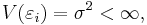
(i.e., all errors have the same variance; that is "homoscedasticity"), and

${\rm cov}(\varepsilon_i,\varepsilon_j) = 0$

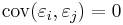
for i ≠ j; that is, any two different values of the error term are drawn from "uncorrelated" distributions. A linear estimator of β_j is a linear combination

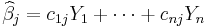
$\widehat\beta_j = c_{1j}Y_1%2B\cdots%2Bc_{nj}Y_n$

in which the coefficients c_ij are not allowed to depend on the underlying coefficients β_j, since those are not observable, but are allowed to depend on the values X_ij, since these data are observable. (The dependence of the coefficients on each X_ij is typically nonlinear; the estimator is linear in each Y_i and hence in each random ε_i, which is why this is "linear" regression.) The estimator is said to be unbiased if and only if

$E(\widehat\beta_j)=\beta_j\,$

regardless of the values of X_ij. Now, let $\sum_{j=1}^K\lambda_j\beta_j$ be some linear combination of the coefficients. Then the mean squared error of the corresponding estimation is

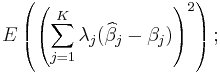
$E \left(\left(\sum_{j=1}^K\lambda_j(\widehat\beta_j-\beta_j)\right)^2\right);$

i.e., it is the expectation of the square of the weighted sum (across parameters) of the differences between the estimators and the corresponding parameters to be estimated. (Since we are considering the case in which all the parameter estimates are unbiased, this mean squared error is the same as the variance of the linear combination.) The best linear unbiased estimator (BLUE) of the vector β of parameters β_j is one with the smallest mean squared error for every vector λ of linear combination parameters. This is equivalent to the condition that

$V(\tilde\beta)- V(\widehat\beta)$

is a positive semi-definite matrix for every other linear unbiased estimator $\tilde\beta$ .

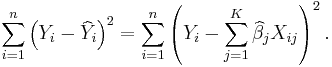
The ordinary least squares estimator (OLS) is the function

$\widehat\beta=(X^{T}X)^{-1}X^{T}Y$

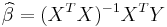
of Y and X that minimizes the sum of squares of residuals (misprediction amounts):

$\sum_{i=1}^n\left(Y_i-\widehat{Y}_i\right)^2=\sum_{i=1}^n\left(Y_i-\sum_{j=1}^K\widehat\beta_j X_{ij}\right)^2.$

The theorem now states that the OLS estimator is a BLUE. The main idea of the proof is that the least-squares estimator is uncorrelated with every linear unbiased estimator of zero, i.e., with every linear combination 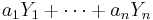$a_1Y_1%2B\cdots%2Ba_nY_n$ whose coefficients do not depend upon the unobservable β but whose expected value is always zero.

Proof

Let $\tilde\beta = CY$ be another linear estimator of $\beta$ and let C be given by 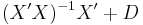$(X'X)^{-1}X' %2B D$ , where D is a $k \times n$ nonzero matrix. As we're restricting to unbiased estimators, minimum mean squared error implies minimum variance. The goal is therefore to show that such an estimator has a variance no smaller than that of $\hat\beta$ , the OLS estimator.

The expectation of $\tilde\beta$ is:

$\begin{align} E(CY) &= E(((X'X)^{-1}X' %2B D)(X\beta %2B \varepsilon)) \\ &= ((X'X)^{-1}X' %2B D)X\beta %2B ((X'X)^{-1}X' %2B D)\underbrace{E(\varepsilon)}_0 \\ &= (X'X)^{-1}X'X\beta %2B DX\beta \\ &= (I_k %2B DX)\beta. \\ \end{align}$

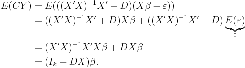
Therefore, $\tilde\beta$ is unbiased if and only if $DX = 0$ .

The variance of $\tilde\beta$ is

$\begin{align} V(\tilde\beta) &= V(CY) = CV(Y)C' = \sigma^2 CC' \\ &= \sigma^2((X'X)^{-1}X' %2B D)(X(X'X)^{-1} %2B D') \\ &= \sigma^2((X'X)^{-1}X'X(X'X)^{-1} %2B (X'X)^{-1}X'D' %2B DX(X'X)^{-1} %2B DD') \\ &= \sigma^2(X'X)^{-1} %2B \sigma^2(X'X)^{-1} (\underbrace{DX}_{0})' %2B \sigma^2 \underbrace{DX}_{0} (X'X)^{-1} %2B \sigma^2DD' \\ &= \underbrace{\sigma^2(X'X)^{-1}}_{V(\hat\beta)} %2B \sigma^2DD'. \end{align}$

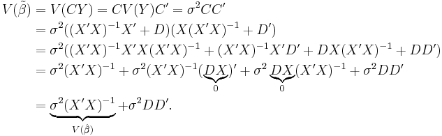
Since DD' is a positive semidefinite matrix, $V(\tilde\beta)$ exceeds $V(\hat\beta)$ by a positive semidefinite matrix.

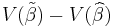
Generalized least squares estimator

The generalized least squares (GLS) or Aitken estimator extends the Gauss–Markov theorem to the case where the error vector has a non-scalar covariance matrix – the Aitken estimator is also a BLUE.^[1]

Notes

^ A. C. Aitken, "On Least Squares and Linear Combinations of Observations", Proceedings of the Royal Society of Edinburgh, 1935, vol. 55, pp. 42–48.

References

Plackett, R.L. (1950). "Some Theorems in Least Squares". Biometrika 37 (1-2): 149–157. doi:10.1093/biomet/37.1-2.149. JSTOR 2332158. MR 36980.

External links

Earliest Known Uses of Some of the Words of Mathematics: G (brief history and explanation of the name)
Proof of the Gauss Markov theorem for multiple linear regression (makes use of matrix algebra)
A Proof of the Gauss Markov theorem using geometry

Least squares and regression analysis

Computational statistics

Least squares · Linear least squares · Non-linear least squares · Iteratively reweighted least squares

Correlation and dependence

Pearson product-moment correlation · Rank correlation (Spearman's rho, Kendall's tau) · Partial correlation · Confounding variable

Regression analysis

Ordinary least squares · Partial least squares · Total least squares · Ridge regression

Regression as a
statistical model

Linear regression	Simple linear regression · Ordinary least squares · Generalized least squares · Weighted least squares · General linear model

Predictor structure	Polynomial regression · Growth curve · Segmented regression · Local regression

Non-standard	Nonlinear regression · Nonparametric · Semiparametric · Robust · Quantile · Isotonic

Non-normal errors	Generalized linear model · Binomial · Poisson · Logistic