B-spline
In the mathematical subfield of numerical analysis, a B-spline is a spline function that has minimal support with respect to a given degree, smoothness, and domain partition. B-splines were investigated as early as the nineteenth century by Nikolai Lobachevsky. A fundamental theorem states that every spline function of a given degree, smoothness, and domain partition, can be uniquely represented as a linear combination of B-splines of that same degree and smoothness, and over that same partition.[1]
The term "B-spline" was coined by Isaac Jacob Schoenberg and is short for basis spline.[2][3] B-splines can be evaluated in a numerically stable way by the de Boor algorithm. Simplified, potentially faster variants of the de Boor algorithm have been created but they suffer from comparatively lower stability.[4][5]
In the computer science subfields of computer-aided design and computer graphics, the term B-spline frequently refers to a spline curve parametrized by spline functions that are expressed as linear combinations of B-splines (in the mathematical sense above). A B-spline is simply a generalisation of a Bézier curve, and it can avoid the Runge phenomenon without increasing the degree of the B-spline.
Contents |
Definition
Given m real values ti, called knots, with
a B-spline of degree n is a parametric curve
![\mathbf{S}:[t_{n}, t_{m-n-1}] \to \mathbb{R}^d](/2012-wikipedia_en_all_nopic_01_2012/I/a8ee34da01bd94da8e8f7a3fb1d41a29.png)
composed of a linear combination of basis B-splines bi,n of degree n
![\mathbf{S}(t)= \sum_{i=0}^{m-n-2} \mathbf{P}_{i} b_{i,n}(t) \mbox{ , } t \in [t_{n},t_{m-n-1}]](/2012-wikipedia_en_all_nopic_01_2012/I/ad3abad98b7261af9e74ad184743f12c.png) .
.
The points  are called control points or de Boor points. There are m−n-1 control points, and they form a convex hull.
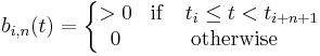
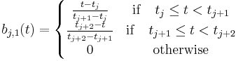
The m-n-1 basis B-splines of degree n can be defined, for n=0,1,...,m-2, using the Cox-de Boor recursion formula

Note that j+n+1 can not exceed m-1, which limits both j and n.
When the knots are equidistant the B-spline is said to be uniform, otherwise non-uniform. If two knots tj are identical, any resulting indeterminate forms 0/0 are deemed to be 0.
Note that when one sums a run of adjacent n-degree basis B-splines one obtains, from this recursion

for any sum with 
When  here, then this sum is, by this recursion, identically equal to 1, within the limited subrange
  , (since this interval excludes the supports of the two basis B-splines in the separate terms at the ends of this sum).
Uniform B-spline
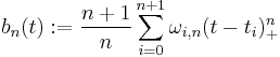
When the B-spline is uniform, the basis B-splines for a given degree n are just shifted copies of each other. An alternative non-recursive definition for the m−n-1 basis B-splines is

with
and
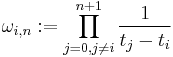
where
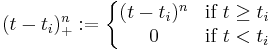
is the truncated power function.
Cardinal B-spline
Define B0 as the characteristic function of ![[-\tfrac{1}{2}, \tfrac{1}{2}]](/2012-wikipedia_en_all_nopic_01_2012/I/19a2ea4a10660560d6779686604a0c8d.png) , and Bk recursively as the convolution product
, and Bk recursively as the convolution product

then Bk are called (centered) cardinal B-splines. This definition goes back to Schoenberg.
Bk has compact support ![[-\tfrac{k%2B1}{2}, \tfrac{k%2B1}{2}]](/2012-wikipedia_en_all_nopic_01_2012/I/49f088871626685ab979ba1845c5a7ee.png) and is an even function. As
and is an even function. As  the normalized cardinal B-splines tend to the Gaussian function.[6]
Notes
When the number of de Boor control points is one more than the degree and  and
and  (thus
(thus ![t \in [0, 1]](/2012-wikipedia_en_all_nopic_01_2012/I/d9a06fde4663cdd5b1ba693e9127232f.png) ), the B-Spline degenerates into a Bézier curve. In particular, the B-Spline basis function
), the B-Spline degenerates into a Bézier curve. In particular, the B-Spline basis function  coincides with the n-th degree univariate Bernstein polynomial.[7] The shape of the basis functions is determined by the position of the knots. Scaling or translating the knot vector does not alter the basis functions.
The spline is contained in the convex hull of its control points.
A basis B-spline of degree n

is non-zero only in the interval [ti, ti+n+1] that is
In other words if we manipulate one control point we only change the local behaviour of the curve and not the global behaviour as with Bézier curves.
Also see Bernstein polynomial for further details.
Examples
Constant B-spline
The constant B-spline is the simplest spline. It is defined on only one knot span and is not even continuous on the knots. It is just the indicator function for the different knot spans.
![b_{j,0}(t) = 1_{[t_j,t_{j%2B1}]} =
\left\{\begin{matrix}
1 & \mathrm{if} \quad t_j \le t < t_{j%2B1} \\
0 & \mathrm{otherwise}
\end{matrix}
\right.](/2012-wikipedia_en_all_nopic_01_2012/I/ccef92716db510a49d8f2d3c47e77e15.png)
Linear B-spline
The linear B-spline is defined on two consecutive knot spans and is continuous on the knots, but not differentiable.
Uniform quadratic B-spline
Quadratic B-splines with uniform knot-vector is a commonly used form of B-spline. The blending function can easily be precalculated, and is equal for each segment in this case.
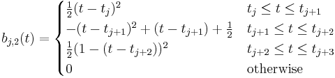
 for
for ![t \in [0,1], i = 1,2 \ldots m-2](/2012-wikipedia_en_all_nopic_01_2012/I/498b8146ef4aa12311e0873d737fd5ab.png)
Cubic B-Spline
A B-spline formulation for a single segment can be written as:
![\mathbf{S}_{i} (t) = \sum_{k=0}^3 \mathbf{P}_{i-3%2Bk} b_{i-3%2Bk,3} (t) \mbox{�; }\ t \in [0,1]](/2012-wikipedia_en_all_nopic_01_2012/I/ed125f5c5449a17aaa556fb6554dca6e.png)
where Si is the ith B-spline segment and P is the set of control points, segment i and k is the local control point index. A set of control points would be 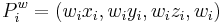 where the
  is weight, pulling the curve towards control point
  as it increases or moving the curve away as it decreases.
An entire set of segments, m-2 curves ( ) defined by m+1 control points (
 ), as one B-spline in t would be defined as:
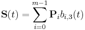
where i is the control point number and t is a global parameter giving knot values. This formulation expresses a B-spline curve as a linear combination of B-spline basis functions, hence the name.
There are two types of B-spline - uniform and non-uniform. A non-uniform B-spline is a curve where the intervals between successive control points are not necessarily equal (the knot vector of interior knot spans are not equal). A common form is where intervals are successively reduced to zero, interpolating control points.
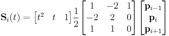
Uniform cubic B-splines
Cubic B-splines with uniform knot-vector is the most commonly used form of B-spline. The blending function can easily be precalculated, and is equal for each segment in this case. Put in matrix-form, it is:
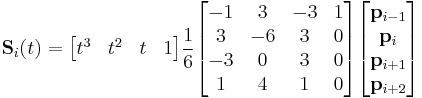
for ![t \in [0,1].](/2012-wikipedia_en_all_nopic_01_2012/I/de4ef1e33d30a0fa6fc661f8fed20bde.png)
See also
References
- ^ Carl de Boor (1978). A Practical Guide to Splines. Springer-Verlag. pp. 113–114.
- ^ Carl de Boor (1978). A Practical Guide to Splines. Springer-Verlag. pp. 114–115.
- ^ Gary D. Knott (2000), Interpolating cubic splines. Springer. p. 151
- ^ Lee, E. T. Y. (December 1982). "A Simplified B-Spline Computation Routine". Computing (Springer-Verlag) 29 (4): 365–371. doi:10.1007/BF02246763.
- ^ Lee, E. T. Y. (1986). "Comments on some B-spline algorithms". Computing (Springer-Verlag) 36 (3): 229–238. doi:10.1007/BF02240069.
- ^ Brinks R: On the convergence of derivatives of B-splines to derivatives of the Gaussian function, Comp. Appl. Math., 27, 1, 2008
- ^ Prautzsch et al., Hartmut (2002). Bezier and B-Spline Techniques. Springer-Verlag. pp. 60–66. ISBN 3540437614.
- ^ Splitting a uniform B-spline curve