Antiderivative
In calculus, an "anti-derivative", antiderivative, primitive integral or indefinite integral[1] of a function f is a function F whose derivative is equal to f, i.e., F ′ = f.[2][3] The process of solving for antiderivatives is called antidifferentiation (or indefinite integration) and its opposite function is called differentiation, which is the process of finding a derivative. Antiderivatives are related to definite integrals through the fundamental theorem of calculus: the definite integral of a function over an interval is equal to the difference between the values of an antiderivative evaluated at the endpoints of the interval.
The discrete equivalent of the notion of antiderivative is antidifference.
Contents |
Example
The function F(x) = x3/3 is an antiderivative of f(x) = x2. As the derivative of a constant is zero, x2 will have an infinite number of antiderivatives; such as (x3/3) + 0, (x3/3) + 7, (x3/3) − 42, (x3/3) + 293 etc. Thus, all the antiderivatives of x2 can be obtained by changing the value of C in F(x) = (x3/3) + C; where C is an arbitrary constant known as the constant of integration. Essentially, the graphs of antiderivatives of a given function are vertical translations of each other; each graph's location depending upon the value of C.
In physics, the integration of acceleration yields velocity plus a constant. The constant is the initial velocity term that would be lost upon taking the derivative of velocity because the derivative of a constant term is zero. This same pattern applies to further integrations and derivatives of motion (position, velocity, acceleration, and so on).
Uses and properties
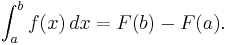
Antiderivatives are important because they can be used to compute definite integrals, using the fundamental theorem of calculus: if F is an antiderivative of the integrable function f, then:
Because of this, each of the infinitely many antiderivatives of a given function f is sometimes called the "general integral" or "indefinite integral" of f and is written using the integral symbol with no bounds:

If F is an antiderivative of f, and the function f is defined on some interval, then every other antiderivative G of f differs from F by a constant: there exists a number C such that G(x) = F(x) + C for all x. C is called the arbitrary constant of integration. If the domain of F is a disjoint union of two or more intervals, then a different constant of integration may be chosen for each of the intervals. For instance
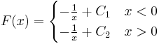
is the most general antiderivative of 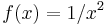 on its natural domain
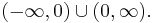
Every continuous function f has an antiderivative, and one antiderivative F is given by the definite integral of f with variable upper boundary:
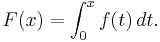
Varying the lower boundary produces other antiderivatives (but not necessarily all possible antiderivatives). This is another formulation of the fundamental theorem of calculus.
There are many functions whose antiderivatives, even though they exist, cannot be expressed in terms of elementary functions (like polynomials, exponential functions, logarithms, trigonometric functions, inverse trigonometric functions and their combinations). Examples of these are

See also differential Galois theory for a more detailed discussion.
Techniques of integration
Finding antiderivatives of elementary functions is often considerably harder than finding their derivatives. For some elementary functions, it is impossible to find an antiderivative in terms of other elementary functions. See the article on elementary functions for further information.
We have various methods at our disposal:
- the linearity of integration allows us to break complicated integrals into simpler ones
- integration by substitution, often combined with trigonometric identities or the natural logarithm
- integration by parts to integrate products of functions
- the inverse chain rule method, a special case of integration by substitution
- the method of partial fractions in integration allows us to integrate all rational functions (fractions of two polynomials)
- the Risch algorithm
- integrals can also be looked up in a table of integrals
- when integrating multiple times, we can use certain additional techniques, see for instance double integrals and polar coordinates, the Jacobian and the Stokes' theorem
- computer algebra systems can be used to automate some or all of the work involved in the symbolic techniques above, which is particularly useful when the algebraic manipulations involved are very complex or lengthy
- if a function has no elementary antiderivative (for instance, exp(-x2)), its definite integral can be approximated using numerical integration
- to calculate the (
 times) repeated antiderivative of a function
  Cauchy's formula is useful (cf. Cauchy formula for repeated integration):

Antiderivatives of non-continuous functions
Non-continuous functions can have antiderivatives. While there are still open questions in this area, it is known that:
- Some highly pathological functions with large sets of discontinuities may nevertheless have antiderivatives.
- In some cases, the antiderivatives of such pathological functions may be found by Riemann integration, while in other cases these functions are not Riemann integrable.
Assuming that the domains of the functions are open intervals:
- A necessary, but not sufficient, condition for a function f to have an antiderivative is that f have the intermediate value property. That is, if [a, b] is a subinterval of the domain of f and d is any real number between f(a) and f(b), then f(c) = d for some c between a and b. To see this, let F be an antiderivative of f and consider the continuous function g(x) = F(x) − dx on the closed interval [a, b]. Then g must have either a maximum or minimum c in the open interval (a, b) and so 0 = g′(c) = f(c) − d.
- The set of discontinuities of f must be a meagre set. This set must also be an F-sigma set (since the set of discontinuities of any function must be of this type). Moreover for any meagre F-sigma set, one can construct some function f having an antiderivative, which has the given set as its set of discontinuities.
- If f has an antiderivative, is bounded on closed finite subintervals of the domain and has a set of discontinuities of Lebesgue measure 0, then an antiderivative may be found by integration.
- If f has an antiderivative F on a closed interval [a,b], then for any choice of partition
 , if one chooses sample points
 ![x_i^*\in[x_{i-1},x_i]](/2012-wikipedia_en_all_nopic_01_2012/I/b20f92b4589859050620eda5dbc80873.png) as specified by the mean value theorem, then the corresponding Riemann sum telescopes to the value F(b) − F(a).
as specified by the mean value theorem, then the corresponding Riemann sum telescopes to the value F(b) − F(a).
![\begin{align}
\sum_{i=1}^n f(x_i^*)(x_i-x_{i-1}) & = \sum_{i=1}^n [F(x_i)-F(x_{i-1})] \\
& = F(x_n)-F(x_0) = F(b)-F(a)
\end{align}](/2012-wikipedia_en_all_nopic_01_2012/I/8c67d903d13b253db42a1f1775aa0685.png)
- However if f is unbounded, or if f is bounded but the set of discontinuities of f has positive Lebesgue measure, a different choice of sample points
 may give a significantly different value for the Riemann sum, no matter how fine the partition. See Example 4 below.
Some examples
- The function
 is not continuous at
  but has the antiderivative
 . Since f is bounded on closed finite intervals and is only discontinuous at 0, the antiderivative F may be obtained by integration:
 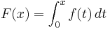 .
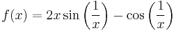
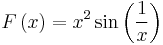
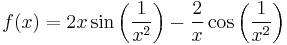
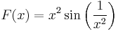
. - The function
is not continuous at but has the antiderivative
. Unlike Example 1, f(x) is unbounded in any interval containing 0, so the Riemann integral is undefined.
- If f(x) is the function in Example 1 and F is its antiderivative, and
 is a dense countable subset of the open interval
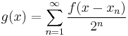
  , then the function
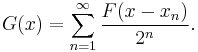
has an antiderivative
The set of discontinuities of g is precisely the set
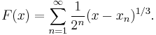
. Since g is bounded on closed finite intervals and the set of discontinuities has measure 0, the antiderivative G may be found by integration. - Let be a dense countable subset of the open interval . Consider the everywhere continuous strictly increasing function
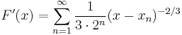
It can be shown that
for all values x where the series converges, and that the graph of F(x) has vertical tangent lines at all other values of x. In particular the graph has vertical tangent lines at all points in the set
.Moreover
 for all x where the derivative is defined. It follows that the inverse function
  is differentiable everywhere and that
for all x in the set
 which is dense in the interval
 ![\left[F\left(-1\right),F\left(1\right)\right]](/2012-wikipedia_en_all_nopic_01_2012/I/af323a0d132aff17d88f037bd32972ed.png) . Thus g has an antiderivative G. On the other hand, it can not be true that
. Thus g has an antiderivative G. On the other hand, it can not be true thatsince for any partition of
, one can choose sample points for the Riemann sum from the set , giving a value of 0 for the sum. It follows that g has a set of discontinuities of positive Lebesgue measure. Figure 1 on the right shows an approximation to the graph of g(x) where  and the series is truncated to 8 terms. Figure 2 shows the graph of an approximation to the antiderivative G(x), also truncated to 8 terms. On the other hand if the Riemann integral is replaced by the Lebesgue integral, then Fatou's lemma or the dominated convergence theorem shows that g does satisfy the fundamental theorem of calculus in that context.
 - In Examples 3 and 4, the sets of discontinuities of the functions g are dense only in a finite open interval
 . However these examples can be easily modified so as to have sets of discontinuities which are dense on the entire real line
  . Let
. Let
 has a dense set of discontinuities on and has antiderivative
- Using a similar method as in Example 5, one can modify g in Example 4 so as to vanish at all rational numbers. If one uses a naive version of the Riemann integral defined as the limit of left-hand or right-hand Riemann sums over regular partitions, one will obtain that the integral of such a function g over an interval
![\left[a,b\right]](/2012-wikipedia_en_all_nopic_01_2012/I/f944498af9d6490b5599ba93146f9db8.png) is 0 whenever a and b are both rational, instead of
is 0 whenever a and b are both rational, instead of 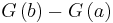 . Thus the fundamental theorem of calculus will fail spectacularly.
See also
Notes
- ^ Antiderivatives are also called general integrals, and sometimes integrals. The latter term is generic, and refers not only to indefinite integrals (antiderivatives), but also to definite integrals. When the word integral is used without additional specification, the reader is supposed to deduce from the context whether it is referred to a definite or indefinite integral. Some authors define the indefinite integral of a function as the set of its infinitely many possible antiderivatives. Others define it as an arbitrarily selected element of that set. Wikipedia adopts the latter approach.
- ^ Stewart, James (2008). Calculus: Early Transcendentals (6th ed.). Brooks/Cole. ISBN 0-495-01166-5.
- ^ Larson, Ron; Edwards, Bruce H. (2009). Calculus (9th ed.). Brooks/Cole. ISBN 0-547-16702-4.
References
- Introduction to Classical Real Analysis, by Karl R. Stromberg; Wadsworth, 1981 (see also)
- Historical Essay On Continuity Of Derivatives, by Dave L. Renfro; http://groups.google.com/group/sci.math/msg/814be41b1ea8c024
External links
- Wolfram Integrator — Free online symbolic integration with Mathematica
- Mathematical Assistant on Web — symbolic computations online. Allows to integrate in small steps (with hints for next step (integration by parts, substitution, partial fractions, application of formulas and others), powered by Maxima
- Function Calculator from WIMS
- Integral
- "The Indefinite Integral or Anti-derivative " at the Khan Academy