Ampère's force law
| Electromagnetism |
|---|
In magnetostatics, the force of attraction or repulsion between two current-carrying wires (see Figure 1) is often called Ampère's force law. The physical origin of this force is that each wire generates a magnetic field, as defined by the Biot-Savart law, and the other wire experiences a magnetic force as a consequence, as defined by the Lorentz force.
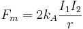
The best-known and simplest example of Ampère's force law, which underlies the definition of the ampere, the SI unit of current, states that the force per unit length between two straight parallel conductors is
-
 ,
,
where kA is the magnetic force constant, r is the separation of the wires, and I1, I2 are the direct currents carried by the wires. This is a good approximation for finite lengths if the distance between the wires is small compared to their lengths, but large compared to their diameters. The value of kA depends upon the system of units chosen, and the value of kA decides how large the unit of current will be. In the SI system,[1] [2]

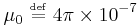
with μ0 the magnetic constant, defined in SI units as[3][4]
Thus, in vacuum, the force per meter of length between two parallel conductors – spaced apart by 1 m and each carrying a current of 1 A – is exactly
-
 N/m.
N/m.
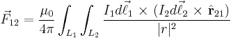
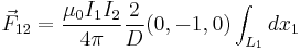
The general formulation of the magnetic force for arbitrary geometries is based on line integrals and combines the Biot-Savart law and Lorentz force in one equation as shown below. [5] [6][7]:
-
 ,
,
where
 is the total force felt by wire 1 due to wire 2 (usually measured in newtons),
- I1 and I2 are the currents running through wires 1 and 2, respectively (usually measured in amperes),
- The double line integration sums the force upon each element of wire 1 due to the magnetic field of each element of wire 2,
 and
and  are infinitesimal vectors associated with wire 1 and wire 2 respectively (usually measured in metres); see line integral for a detailed definition,
- The vector
 is the unit vector pointing from the differential element on wire 2 towards the differential element on wire 1, and |r| is the distance separating these elements,
 - The multiplication × is a vector cross product,
- The sign of In is relative to the orientation
 (for example, if points in the direction of conventional current, then I1>0).
To determine the force between wires in a material medium, the magnetic constant is replaced by the actual permeability of the medium.
Contents |
Historical Background
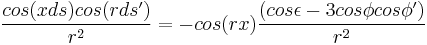
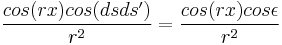
The form of Ampere's force law commonly given was derived by Maxwell and is one of several expressions consistent with the original experiments of Ampere and Gauss. The x-component of the force between two linear currents I and I’, as depicted in the diagram to the right, was given by Ampere in 1825 and Gauss in 1833 as follows[8] :
-
 .
.
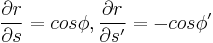
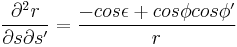
Following Ampere, a number of scientists, including Wilhelm Weber, Rudolf Clausius, James Clerk Maxwell, Bernhard Riemann and Walter Ritz, developed this expression to find a fundamental expression of the force. Through differentiation, it can be shown that:
-
 .
.
and also the identity:
-
 .
.
With these expressions, Ampere's force law can be expressed as:
-
 .
.
Using the identities:
-
 .
.
and
-
 .
.
Ampere's results can be expressed in the form:
-
 .
.
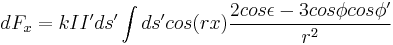
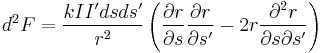
As Maxwell noted, terms can be added to this expression, which are derivatives of a function Q(r) and, when integrated, cancel each other out. Thus, Maxwell gave "the most general form consistent with the experimental facts" for the force on ds arising from the action of ds'[9] :
-
![d^2 F_x = k I I' ds ds' \left[ \left( \frac{1} {r^2} \left( \frac{\partial r}{\partial s} \frac{\partial r}{\partial s'} - 2r \frac{\partial^2 r}{\partial s \partial s'}\right) %2B r \frac{\partial^2 Q}{\partial s \partial s'}\right) cos(rx) %2B \frac{\partial Q} {\partial s'} cos(xds) - \frac{\partial Q} {\partial s} cos(xds') \right]](/2012-wikipedia_en_all_nopic_01_2012/I/6a2b732f47b6aaa14920f9b679d6ed25.png) .
.
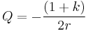
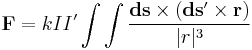
Q is a function of r, according to Maxwell, which "cannot be determined, without assumptions of some kind, from experiments in which the active current forms a closed circuit." Taking the function Q(r) to be of the form:
We obtain the general expression for the force exerted on ds by ds:
-
![\mathbf{d^2F} = -\frac{k I I'} {2r^2} \left[ (3-k)\hat{\mathbf{r_1}} (\mathbf{dsds'}) - 3(1-k) \hat{\mathbf{r_1}} (\mathbf{\hat{r_1} ds}) (\mathbf{\hat{r_1} ds'}) - (1%2Bk)\mathbf{ds} (\mathbf{\hat{r_1} ds'})-(1%2Bk) \mathbf{d's} (\mathbf{\hat{r_1} ds}) \right]](/2012-wikipedia_en_all_nopic_01_2012/I/d8175f96f0833960ab870b1bac228b59.png) .
.
Integrating around s' eliminates k and the original expression given by Ampere and Gauss is obtained. Thus, as far as the original Ampere experiments are concerned, the value of k has no significance. Ampere took k=-1; Gauss took k=+1, as did Grassmann and Clausius, although Clausius omitted the S component. In the non-etheral electron theories, Weber took k=-1 and Riemann took k=+1. Ritz left k undetermined in his theory. If we take k = -1, we obtain the Ampere expression:
![\mathbf{d^2F} = -\frac{k I I'} {r^3} \left[ 2 \mathbf{r} (\mathbf{dsds'}) - 3\mathbf{r} (\mathbf{r ds}) (\mathbf{r ds'}) \right]](/2012-wikipedia_en_all_nopic_01_2012/I/ce87e52854d350c8562ebdab893ab4a3.png)
If we take k=+1, we obtain
![\mathbf{d^2F} = -\frac{k I I'} {r^3} \left[ \mathbf{r} (\mathbf{dsds'}) - \mathbf{ds (r ds')} -\mathbf{ds'(r ds)} \right]](/2012-wikipedia_en_all_nopic_01_2012/I/5d5f1d7a36d88e7fe7d600f9b61d4973.png)
Using the vector identity for the triple cross product, we may express this result as
![\mathbf{d^2F} = \frac{k I I'} {r^3} \left[ \left(\mathbf{ds}\times\mathbf{ds'}\times\mathbf{r}\right)%2B \mathbf{ds'(r ds)} \right]](/2012-wikipedia_en_all_nopic_01_2012/I/874d475e8445cf5d0180e2b6a6006c6f.png)
When integrated around ds' the second term is zero, and thus we find the form of Ampere's force law given by Maxwell:
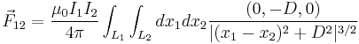
Derivation of parallel straight wire case from general formula
Start from the general formula:
-
- ,
Assume wire 2 is along the x-axis, and wire 1 is at y=D, z=0, parallel to the x-axis. Let  be the x-coordinate of the differential element of wire 1 and wire 2, respectively. In other words, the differential element of wire 1 is at
  and the differential element of wire 2 is at
  . By properties of line integrals,
 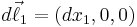 and
and 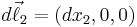 . Also,
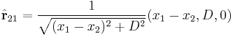
and
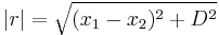
Therefore the integral is
-
 .
.
Evaluating the cross-product:
-
 .
.
Next, we integrate  from
from  to
to  :
:
-
 .
.
If wire 1 is also infinite, the integral diverges, because the total attractive force between two infinite parallel wires is infinity. In fact, we want to know the attractive force per unit length of wire 1. Therefore, assume wire 1 has a large but finite length  . Then the force vector felt by wire 1 is:
-
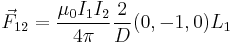 .
.
As expected, the force that the wire feels is proportional to its length. The force per unit length is:
-
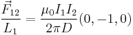 .
.
The direction of the force is along the y-axis, representing wire 1 getting pulled towards wire 2 if the currents are parallel, as expected. The magnitude of the force per unit length agrees with the expression for  shown above.
References and notes
- ^ Raymond A Serway & Jewett JW (2006). Serway's principles of physics: a calculus based text (Fourth Edition ed.). Belmont, CA: Thompson Brooks/Cole. p. 746. ISBN 053449143X. http://books.google.com/books?id=1DZz341Pp50C&pg=RA1-PA746&dq=wire+%22magnetic+force%22&lr=&as_brr=0&sig=4vMV_CH6Nm8ZkgjtDJFlupekYoA#PRA1-PA746,M1.
- ^ Paul M. S. Monk (2004). Physical chemistry: understanding our chemical world. New York: Chichester: Wiley. p. 16. ISBN 0471491810. http://books.google.com/books?vid=ISBN0471491802&id=LupAi35QjhoC&pg=PA16&lpg=PA16&ots=IMiGyIL-67&dq=ampere+definition+si&sig=9Y0k0wgvymmLNYFMcXodwJZwvAM.
- ^ BIPM definition
- ^ "Magnetic constant". 2006 CODATA recommended values. NIST. http://physics.nist.gov/cgi-bin/cuu/Value?mu0. Retrieved 2007-08-08.
- ^ The integrand of this expression appears in the official documentation regarding definition of the ampere BIPM SI Units brochure, 8th Edition, p. 105
- ^ Tai L. Chow (2006). Introduction to electromagnetic theory: a modern perspective. Boston: Jones and Bartlett. p. 153. ISBN 0763738271. http://books.google.com/books?id=dpnpMhw1zo8C&pg=PA153&lpg=PA153&dq=%22ampere's+law+of+force%22&source=web&ots=uZOFz9dWv7&sig=NJp3UQvbCOvcVm7eJN4IUdlC9bs.
- ^ Ampère's Force Law Scroll to section "Integral Equation" for formula.
- ^ O'Rahilly, Alfred (1965). Electromagnetic Theory. Dover. pp. 104.
- ^ Maxwell, James Clerk (1904). Treatise on Electricity and Magnetism. Oxford. pp. 173.
Further reading
- Ampère's force law Includes animated graphic of the force vectors.