Affine transformation

In geometry, an affine transformation or affine map ^[1] or an affinity (from the Latin, affinis, "connected with") is a transformation which preserves straight lines. (i.e., all points lying on a line initially still lie on a line after transformation) and ratios of distances (e.g., the midpoint of a line segment remains the midpoint after transformation). While an affine transformation preserves proportions on lines, it does not necessarily preserve angles or lengths. It is the most general class of transformations with this property. Geometric contraction, expansion, dilation, reflection, rotation, shear, similarity transformations, spiral similarities, and translation are all affine transformations, as are their combinations. It is equivalent to a translation followed by a linear transformation.

1 Mathematical Definition
2 Representation
3 Properties
4 Affine transformation of the plane
5 Examples of affine transformations
- 5.1 Affine transformation over a finite field
- 5.2 Affine transformation in plane geometry
6 See also
7 Notes
8 References
9 External links

Mathematical Definition

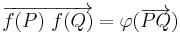
An affine map $\scriptstyle f:\mathcal{A} \;\to\; \mathcal{B}$ between two affine spaces is a map that acts on vectors, defined by pairs of points, as a linear transformation: there exists a linear transformation φ such that

$\overrightarrow{f(P)~f(Q)} = \varphi(\overrightarrow{PQ})$

for any pair of points $\scriptstyle P,\, Q \,\in\, \mathcal{A}$ . If an origin $\scriptstyle O \in \mathcal{A}$ is chosen, and $\scriptstyle B\,$ denotes its image $\scriptstyle f(O) \,\in\, \mathcal{B}$ , then this means that for any vector $\scriptstyle \vec{x}$ :

$f: O%2B\vec{x} \mapsto B%2B\varphi(\vec{x}).$

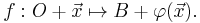
If an origin $\scriptstyle O' \,\in\, \mathcal{B}$ is also chosen, this can be decomposed as an affine transformation $\scriptstyle \mathcal{A} \,\to\, \mathcal{B}$ that sends $\scriptstyle O \;\mapsto\; O'$ , namely

$f: O%2B\vec{x} \mapsto O'%2B\varphi(\vec{x})$

followed by the translation by a vector $\scriptstyle \vec{b} \;=\; \overrightarrow{O'B}$ .

The conclusion is that, heuristically, $\scriptstyle f$ consists of a translation and a linear map.

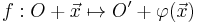
Another definition is: Given two affine spaces $\scriptstyle \mathcal{A}$ and $\scriptstyle \mathcal{B}$ , over the same field, a function $\scriptstyle f:\, \mathcal{A} \;\to\; \mathcal{B}$ is an affine map if and only if for every family $\scriptstyle \{(a_i,\, \lambda_i)\}_{i\in I}\,$ of weighted points in $\scriptstyle \mathcal{A}$ such that $\scriptstyle \sum_{i\in I}\lambda_i \;=\; 1\, ,$ we have

$f\left(\sum_{i\in I}\lambda_i a_i\right)=\sum_{i\in I}\lambda_i f(a_i)\, .$

In other words, $\scriptstyle f\,$ preserves barycenters.

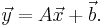
In the finite-dimensional case, an affine map can be specified in coordinates by a matrix A (describing φ) together with the vector $\scriptstyle \vec{b}$ .

An affine transformation preserves

The collinearity relation between points; i.e., the points which lie on a line continue to be collinear after the transformation
Ratios of vectors along a line; i.e., for distinct collinear points $\scriptstyle p_1,\, p_2,\, p_3,$ the ratio of $\scriptstyle \overrightarrow{p_1p_2}$ and $\scriptstyle \overrightarrow{p_2p_3}$ is the same as that of $\scriptstyle \overrightarrow{f(p_1)f(p_2)}$ and $\scriptstyle \overrightarrow{f(p_2)f(p_3)}$ .
More generally barycenters of weighted collections of points.

Representation

Ordinary vector algebra uses matrix multiplication to represent linear transformations, and vector addition to represent translations. Using an augmented matrix and an augmented vector, it is possible to represent both using a single matrix multiplication. The technique requires that all vectors are augmented with a "1" at the end, and all matrices are augmented with an extra row of zeros at the bottom, an extra column—the translation vector—to the right, and a "1" in the lower right corner. If A is a matrix,

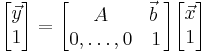
$\begin{bmatrix} \vec{y} \\ 1 \end{bmatrix} = \begin{bmatrix} A & \vec{b} \ \\ 0, \ldots, 0 & 1 \end{bmatrix} \begin{bmatrix} \vec{x} \\ 1 \end{bmatrix}$

is equivalent to the following

$\vec{y} = A \vec{x} %2B \vec{b}.$

The above mentioned augmented matrix is called affine transformation matrix, or projective transformation matrix (as it can also be used to perform Projective transformations).

This representation exhibits the set of all invertible affine transformations as the semidirect product of Kⁿ and GL(n, k). This is a group under the operation of composition of functions, called the affine group.

Ordinary matrix-vector multiplication always maps the origin to the origin, and could therefore never represent a translation, in which the origin must necessarily be mapped to some other point. By appending the additional coordinate "1" to every vector, one essentially considers the space to be mapped as a subset of a space with an additional dimension. In that space, the original space occupies the subset in which the additional coordinate is 1. Thus the origin of the original space can be found at (0,0, ... 0, 1). A translation within the original space by means of a linear transformation of the higher-dimensional space is then possible (specifically, a shear transformation). The coordinates in the higher-dimensional space are an example of homogeneous coordinates. If the original space is Euclidean, the higher dimensional space is a real projective space.

The advantage of using homogeneous coordinates is that one can combine any number of affine transformations into one by multiplying the respective matrices. This property is used extensively in computer graphics.

Properties

An affine transformation is invertible if and only if A is invertible. In the matrix representation, the inverse is:

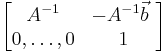
$\begin{bmatrix} A^{-1} & -A^{-1}\vec{b} \ \\ 0,\ldots,0 & 1 \end{bmatrix}$

The invertible affine transformations (of an affine space onto itself) form the affine group, which has the general linear group of degree n as subgroup and is itself a subgroup of the general linear group of degree n + 1.

The similarity transformations form the subgroup where A is a scalar times an orthogonal matrix. If and only if the determinant of A is 1 or −1 then the transformation is an equi-areal mapping. Such transformations form a subgroup called the equi-affine group^[2]

Combining both conditions we have the isometries, the subgroup of both where A is an orthogonal matrix.

Each of these groups has a subgroup of transformations which preserve orientation: those where the determinant of A is positive. In the last case this is in 3D the group of rigid body motions (proper rotations and pure translations).

For any matrix A the following propositions are equivalent:

A − I is invertible
A does not have an eigenvalue equal to 1
for all b the transformation has exactly one fixed point
there is a b for which the transformation has exactly one fixed point
affine transformations with matrix A can be written as a linear transformation with some point as origin

If there is a fixed point, we can take that as the origin, and the affine transformation reduces to a linear transformation. This may make it easier to classify and understand the transformation. For example, describing a transformation as a rotation by a certain angle with respect to a certain axis is easier to get an idea of the overall behavior of the transformation than describing it as a combination of a translation and a rotation. However, this depends on application and context. Describing such a transformation for an object tends to make more sense in terms of rotation about an axis through the center of that object, combined with a translation, rather than by just a rotation with respect to some distant point. As an example: "move 200 m north and rotate 90° anti-clockwise", rather than the equivalent "with respect to the point 141 m to the northwest, rotate 90° anti-clockwise".

Affine transformations in 2D without fixed point (so where A has eigenvalue 1) are:

pure translations
scaling in a given direction, with respect to a line in another direction (not necessarily perpendicular), combined with translation that is not purely in the direction of scaling; the scale factor is the other eigenvalue; taking "scaling" in a generalized sense it includes the cases that the scale factor is zero (projection) and negative; the latter includes reflection, and combined with translation it includes glide reflection.
shear combined with translation that is not purely in the direction of the shear (there is no other eigenvalue than 1; it has algebraic multiplicity 2, but geometric multiplicity 1)

Affine transformation of the plane

To visualise the general affine transformation of the Euclidean plane, take labelled parallelograms ABCD and A′B′C′D′. Whatever the choices of points, there is an affine transformation T of the plane taking A to A′, and each vertex similarly. Supposing we exclude the degenerate case where ABCD has zero area, there is a unique such affine transformation T. Drawing out a whole grid of parallelograms based on ABCD, the image T(P) of any point P is determined by noting that T(A) = A′, T applied to the line segment AB is A′B′, T applied to the line segment AC is A′C′, and T respects scalar multiples of vectors based at A. [If A, E, F are collinear then the ratio length(AF)/length(AE) is equal to length(A′F′)/length(A′E′).] Geometrically T transforms the grid based on ABCD to that based in A′B′C′D′.

Affine transformations don't respect lengths or angles; they multiply area by a constant factor

area of A′B′C′D′ / area of ABCD.

A given T may either be direct (respect orientation), or indirect (reverse orientation), and this may be determined by its effect on signed areas (as defined, for example, by the cross product of vectors).

Examples of affine transformations

Affine transformation over a finite field

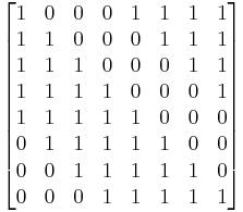
The following equation expresses an affine transformation in GF(2⁸) (with "+" representing XOR):

$\{\,a'\,\} = M\{\,a\,\} %2B \{\,v\,\},$

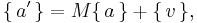
where [M] is the matrix

$\begin{bmatrix} 1&0&0&0&1&1&1&1 \\ 1&1&0&0&0&1&1&1 \\ 1&1&1&0&0&0&1&1 \\ 1&1&1&1&0&0&0&1 \\ 1&1&1&1&1&0&0&0 \\ 0&1&1&1&1&1&0&0 \\ 0&0&1&1&1&1&1&0 \\ 0&0&0&1&1&1&1&1 \end{bmatrix}$

and {v} is the vector

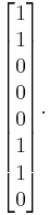
$\begin{bmatrix} 1 \\ 1 \\ 0 \\ 0 \\ 0 \\ 1 \\ 1 \\ 0 \end{bmatrix}.$

For instance, the affine transformation of the element {a} = y⁷ + y⁶ + y³ + y = {11001010} in big-endian binary notation = {CA} in big-endian hexadecimal notation, is calculated as follows:

$a_0' = a_0 \oplus a_4 \oplus a_5 \oplus a_6 \oplus a_7 \oplus 1 = 0 \oplus 0 \oplus 0 \oplus 1 \oplus 1 \oplus 1 = 1$

$a_1' = a_0 \oplus a_1 \oplus a_5 \oplus a_6 \oplus a_7 \oplus 1 = 0 \oplus 1 \oplus 0 \oplus 1 \oplus 1 \oplus 1 = 0$

$a_2' = a_0 \oplus a_1 \oplus a_2 \oplus a_6 \oplus a_7 \oplus 0 = 0 \oplus 1 \oplus 0 \oplus 1 \oplus 1 \oplus 0 = 1$

$a_3' = a_0 \oplus a_1 \oplus a_2 \oplus a_3 \oplus a_7 \oplus 0 = 0 \oplus 1 \oplus 0 \oplus 1 \oplus 1 \oplus 0 = 1$

$a_4' = a_0 \oplus a_1 \oplus a_2 \oplus a_3 \oplus a_4 \oplus 0 = 0 \oplus 1 \oplus 0 \oplus 1 \oplus 0 \oplus 0 = 0$

$a_5' = a_1 \oplus a_2 \oplus a_3 \oplus a_4 \oplus a_5 \oplus 1 = 1 \oplus 0 \oplus 1 \oplus 0 \oplus 0 \oplus 1 = 1$

$a_6' = a_2 \oplus a_3 \oplus a_4 \oplus a_5 \oplus a_6 \oplus 1 = 0 \oplus 1 \oplus 0 \oplus 0 \oplus 1 \oplus 1 = 1$

$a_7' = a_3 \oplus a_4 \oplus a_5 \oplus a_6 \oplus a_7 \oplus 0 = 1 \oplus 0 \oplus 0 \oplus 1 \oplus 1 \oplus 0 = 1.$

Thus, {a′} = y⁷ + y⁶ + y⁵ + y³ + y² + 1 = {11101101} = {ED}.

Affine transformation in plane geometry

In ℝ², the transformation shown at right is accomplished using the map given by:

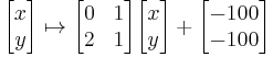
$\begin{bmatrix} x \\ y\end{bmatrix} \mapsto \begin{bmatrix} 0&1\\ 2&1 \end{bmatrix}\begin{bmatrix} x \\ y\end{bmatrix} %2B \begin{bmatrix} -100 \\ -100\end{bmatrix}$

Transforming the three corner points of the original triangle (in red) gives three new points which form the new triangle (in blue). This transformation skews and translates the original triangle.

In fact, all triangles are related to one another by affine transformations. This is also true for all parallelograms, but not for all quadrilaterals.

Notes

^ Berger, Marcel (1987), p. 38
^ Oswald Veblen and John Wesley Young (1918) Projective Geometry, volume 2, page 105–7

References

Berger, Marcel (1987), Geometry I, Berlin: Springer, ISBN 3-540-11658-3
Nomizu, K.; Sasaki, S. (1994), Affine Differential Geometry (New ed.), Cambridge University Press, ISBN 9780521441773
Sharpe, R. W. (1997). Differential Geometry: Cartan's Generalization of Klein's Erlangen Program. New York: Springer. ISBN 0-387-94732-9.

External links

Geometric Operations: Affine Transform, R. Fisher, S. Perkins, A. Walker and E. Wolfart.
Weisstein, Eric W., "Affine Transformation" from MathWorld.
Affine Transform by Bernard Vuilleumier, Wolfram Demonstrations Project.
Affine Transformation on PlanetMath
Free Affine Transformation software