Chebyshev's inequality

In probability theory, Chebyshev's inequality (also known as Tchebysheff's inequality, Chebyshev's theorem, or the Bienaymé–Chebyshev inequality) guarantees that in any data sample or probability distribution, "nearly all" the values are "close to" the mean value — the precise statement being that no more than 1/k² of the distribution's values can be more than k standard deviations away from the mean. The inequality has great utility because it can be applied to completely arbitrary distributions (unknown except for mean and variance), and is a step in the proof of the weak law of large numbers.

The theorem is named for the Russian mathematician Pafnuty Chebyshev, although it was first formulated by his friend and colleague Irénée-Jules Bienaymé.^[1] It can be stated quite generally using measure theory; the statement in the language of probability theory then follows as a particular case, for a space of measure 1.

The term "Chebyshev's inequality" may also refer to Markov's inequality, especially in the context of analysis.

1 Statement
- 1.1 Measure-theoretic statement
- 1.2 Probabilistic statement
2 Variant: One-sided Chebyshev inequality
- 2.1 An application: distance between the mean and the median
  - 2.1.1 Proof using Chebyshev's inequality
  - 2.1.2 Proof using Jensen's inequality
3 Proof (of the two-sided Chebyshev's inequality)
- 3.1 Measure-theoretic proof
- 3.2 Probabilistic proof
4 See also
5 References
6 Further reading

Statement

Measure-theoretic statement

Let (X, Σ, μ) be a measure space, and let ƒ be an extended real-valued measurable function defined on X. Then for any real number t > 0,

$\mu(\{x\in X\,:\,\,|f(x)|\geq t\}) \leq {1\over t^2} \int_X f^2 \, d\mu.$

More generally, if g is a nonnegative extended real-valued measurable function, nondecreasing on the range of ƒ, then

$\mu(\{x\in X\,:\,\,f(x)\geq t\}) \leq {1\over g(t)} \int_X g\circ f\, d\mu.$

The previous statement then follows by defining g(t) as

$g(t)=\begin{cases}t^2&\mbox{if }t\geq0\\0&\mbox{otherwise,}\end{cases}$

and taking |ƒ| instead of ƒ.

Probabilistic statement

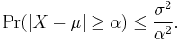
Let X be a random variable with expected value μ and finite variance σ². Then for any real number k > 0,

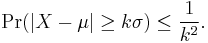
$\Pr(\left|X-\mu\right|\geq k\sigma)\leq\frac{1}{k^2}.$

Only the cases k > 1 provide useful information. This can be equivalently stated as

$\Pr(\left|X-\mu\right|\geq \alpha)\leq\frac{\sigma^2}{\alpha^2}.$

As an example, using k = √2 shows that at least half of the values lie in the interval (μ − √2 σ, μ + √2 σ).

Because it can be applied to completely arbitrary distributions (unknown except for mean and variance), the inequality gives a poor bound compared to what might be possible if something is known about the distribution involved.

For example, suppose we have a pile of journal articles which are on average 1000 words long, with a standard deviation of 200 words. We can then infer that of these articles, the proportion which are between 600 and 1400 words (i.e. within k = 2 SDs of the mean) cannot be less than 3/4, because no more than 1/k² = 1/4 lie outside that range, by Chebyshev's inequality. But if we additionally know that the distribution is normal, we can say that 75% of the values are between 770 and 1230 (which is of course a tighter bound than that given a moment ago).

As demonstrated in the example above, the theorem will typically provide rather loose bounds. However, the bounds provided by Chebyshev's inequality cannot, in general (remaining sound for variables of arbitrary distribution), be improved upon. For example, for any k > 1, the following example (where σ = 1/k) meets the bounds exactly.

$\begin{align} & {} \Pr(X=-1) = \frac{1}{2k^2}, \\ & {} \Pr(X=0) = 1 - \frac{1}{k^2}, \\ & {} \Pr(X=1) = \frac{1}{2k^2}. \end{align}$

For this distribution,

$\mathrm{Pr}\left(\left|X-\mu\right| \ge k\sigma\right) = \frac{1}{k^2}.$

Equality holds exactly for any distribution that is a linear transformation of this one. Inequality holds for any distribution that is not a linear transformation of this one.

Variant: One-sided Chebyshev inequality

A one-tailed variant with k > 0, is^[2]

$\Pr(X-\mu \geq k\sigma)\leq\frac{1}{1+k^2}.$

The one-sided version of the Chebyshev inequality is called Cantelli's inequality, and is due to Francesco Paolo Cantelli.

An application: distance between the mean and the median

The one-sided variant can be used to prove the proposition that for probability distributions having an expected value and a median, the mean (i.e., the expected value) and the median can never differ from each other by more than one standard deviation. To express this in mathematical notation, let μ, m, and σ be respectively the mean, the median, and the standard deviation. Then

$\left|\mu-m\right| \leq \sigma. \,$

(There is no need to rely on an assumption that the variance exists, i.e., is finite. Unlike the situation with the expected value, saying the variance exists is equivalent to saying the variance is finite. But this inequality is trivially true if the variance is infinite.)

Proof using Chebyshev's inequality

Setting k = 1 in the statement for the one-sided inequality gives:

$\Pr(X-\mu \geq \sigma)\leq\frac{1}{2}.$

By changing the sign of X and so of μ, we get

$\Pr(X \leq \mu - \sigma) \leq\frac{1}{2}.$

Thus the median is within one standard deviation of the mean.

Proof using Jensen's inequality

This proof uses Jensen's inequality twice. We have

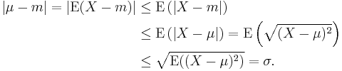
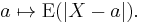
$\begin{align} \left|\mu-m\right| = \left|\mathrm{E}(X-m)\right| & {} \leq \mathrm{E}\left(\left|X-m\right|\right) \\ & {} \leq \mathrm{E}\left(\left|X-\mu\right|\right) = \mathrm{E}\left(\sqrt{(X-\mu)^2}\right) \\ & {} \leq \sqrt{\mathrm{E}((X-\mu)^2)} = \sigma. \end{align}$

The first inequality comes from (the convex version of) Jensen's inequality applied to the absolute value function, which is convex. The second comes from the fact that the median minimizes the absolute deviation function

$a \mapsto \mathrm{E}(\left|X-a\right|).\,$

The third inequality comes from (the concave version of) Jensen's inequality applied to the square root function, which is concave. Q.E.D.

Proof (of the two-sided Chebyshev's inequality)

Measure-theoretic proof

Let A_t be defined as A_t := {x ∈ X | ƒ(x) ≥ t}, and let 1_{A_t} be the indicator function of the set A_t. Then, it is easy to check that

$0\leq g(t) 1_{A_t}\leq g\circ f\,1_{A_t}\leq g\circ f,$

and therefore,

$g(t)\mu(A_t)=\int_X g(t)1_{A_t}\,d\mu\leq\int_{A_t} g\circ f\,d\mu\leq\int_X g\circ f\,d\mu.$

The desired inequality follows from dividing the above inequality by g(t).

Probabilistic proof

Markov's inequality states that for any real-valued random variable Y and any positive number a, we have Pr(|Y| > a) ≤ E(|Y|)/a. One way to prove Chebyshev's inequality is to apply Markov's inequality to the random variable Y = (X − μ)² with a = (σk)².

It can also be proved directly. For any event A, let I_A be the indicator random variable of A, i.e. I_A equals 1 if A occurs and 0 otherwise. Then

$\begin{align} & {} \qquad \Pr(|X-\mu| \geq k\sigma) = \operatorname{E}(I_{|X-\mu| \geq k\sigma}) = \operatorname{E}(I_{[(X-\mu)/(k\sigma)]^2 \geq 1}) \\[6pt] & \leq \operatorname{E}\left( \left( {X-\mu \over k\sigma} \right)^2 \right) = {1 \over k^2} {\operatorname{E}((X-\mu)^2) \over \sigma^2} = {1 \over k^2}. \end{align}$

The direct proof shows why the bounds are quite loose in typical cases: the number 1 to the left of "≥" is replaced by [(X − μ)/(kσ)]² to the right of "≥" whenever the latter exceeds 1. In some cases it exceeds 1 by a very wide margin.

References

↑ Donald Knuth, "The Art of Computer Programming", 3rd ed., vol. 1, 1997, p.98
↑ Grimmett and Stirzaker, problem 7.11.9. Several proofs of this result can be found here.