WKB approximation
In physics, the WKB (Wentzel–Kramers–Brillouin) approximation, also known as WKBJ (Wentzel–Kramers–Brillouin–Jeffreys) approximation, is the most familiar example of a semiclassical calculation in quantum mechanics in which the wavefunction is recast as an exponential function, semiclassically expanded, and then either the amplitude or the phase is taken to be slowly changing.
Contents |
Brief history
This method is named after physicists Wentzel, Kramers, and Brillouin, who all developed it in 1926. In 1923, mathematician Harold Jeffreys had developed a general method of approximating linear, second-order differential equations, which includes the Schrödinger equation. But since the Schrödinger equation was developed two years later, and Wentzel, Kramers, and Brillouin were apparently unaware of this earlier work, Jeffreys is often neglected credit. Early texts in quantum mechanics contain any number of combinations of their initials, including WBK, BWK, WKBJ and BWKJ.
Earlier references to the method are: Carlini in 1817, Liouville in 1837, Green in 1837, Rayleigh in 1912 and Gans in 1915. Liouville and Green may be called the founders of the method, in 1837.
The important contribution of Wentzel, Kramers, Brillouin and Jeffreys to the method was the inclusion of the treatment of turning points, connecting the evanescent and oscillatory solutions at either side of the turning point. For example, this may occur in the Schrödinger equation, due to a potential energy hill.
WKB method
Generally, WKB theory is a method for approximating the solution of a differential equation whose highest derivative is multiplied by a small parameter ε. The method of approximation is as follows:
For a differential equation

assume a solution of the form of an asymptotic series expansion
![y(x) \sim \exp\left[\frac{1}{\delta}\sum_{n=0}^{\infty}\delta^nS_n(x)\right]](/2009-wikipedia_en_wp1-0.7_2009-05/I/0a264fde83815498bd4d33fd6753959d.png)
In the limit  . Substitution of the above ansatz into the differential equation and canceling out the exponential terms allows one to solve for an arbitrary number of terms
  in the expansion. WKB Theory is a special case of Multiple Scale Analysis.
An example
Consider the second-order homogeneous linear differential equation
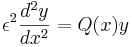
where  . Plugging in
![y(x) = \exp\left[\frac{1}{\delta}\sum_{n=0}^{\infty}\delta^nS_n(x)\right]](/2009-wikipedia_en_wp1-0.7_2009-05/I/a7c9b8bcb8c0651ee5bb7185710c09a4.png)
results in the equation
![\epsilon^2\left[\frac{1}{\delta^2}\left(\sum_{n=0}^{\infty}\delta^nS_n'\right)^2 + \frac{1}{\delta}\sum_{n=0}^{\infty}\delta^nS_n''\right] = Q(x)](/2009-wikipedia_en_wp1-0.7_2009-05/I/de233b64244da7ea29b7dc3266464a92.png)
To leading order, (assuming, for the moment, the series will be asymptotically consistent) the above can be approximated as
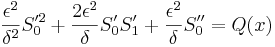
In the limit , the dominant balance is given by

So δ is proportional to ε. Setting them equal and comparing powers renders
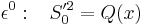
Which can be recognized as the Eikonal equation, with solution
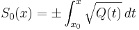
Looking at first-order powers of  gives
gives
Which is the unidimensional transport equation, which has the solution

And  is an arbitrary constant. We now have a pair of approximations to the system (a pair because
  can take two signs); the first-order WKB-approximation will be a linear combination of the two:
![y(x) \approx c_1Q^{-\frac{1}{4}}(x)\exp\left[\frac{1}{\epsilon}\int_{x_0}^x\sqrt{Q(t)}dt\right] + c_2Q^{-\frac{1}{4}}(x)\exp\left[-\frac{1}{\epsilon}\int_{x_0}^x\sqrt{Q(t)}dt\right]](/2009-wikipedia_en_wp1-0.7_2009-05/I/6d2ae4906b48bd56556e5955c3d88cec.png)
Higher-order terms can be obtained by looking at equations for higher powers of ε. Explicitly
for  . This example comes from Bender and Orszag's textbook (see references).
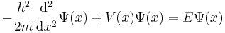
Application to Schrödinger equation
The one dimensional, time-independent Schrödinger equation is
 ,
,
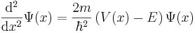
which can be rewritten as
 .
.
The wavefunction can be rewritten as the exponential of another function Φ (which is closely related to the action):
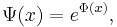
so that
![\Phi''(x) + \left[\Phi'(x)\right]^2 = \frac{2m}{\hbar^2} \left( V(x) - E \right),](/2009-wikipedia_en_wp1-0.7_2009-05/I/0d38c13053c74bca8408f53ba53b6866.png)
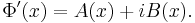
where Φ' indicates the derivative of Φ with respect to x. The derivative  can be separated into real and imaginary parts by introducing the real functions A and B:
The amplitude of the wavefunction is then  , while the phase is
  . The Schrödinger equation implies that these functions must satisfy:
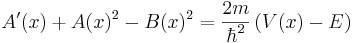
and therefore, since the right hand side of the differential equation for Φ is real,

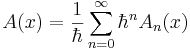
Next, the semiclassical approximation is invoked. This means that each function is expanded as a power series in  . From the equations it can be seen that the power series must start with at least an order of
  to satisfy the real part of the equation. In order to achieve a good classical limit, it is necessary to start with as high a power of Planck's constant as possible.
To first order in this expansion, the conditions on A and B can be written.

If the amplitude varies sufficiently slowly as compared to the phase ( ), it follows that

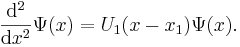
which is only valid when the total energy is greater than the potential energy, as is always the case in classical motion. After the same procedure on the next order of the expansion it follows that
![\Psi(x) \approx C_0 \frac{ e^{i \int \mathrm{d}x \sqrt{\frac{2m}{\hbar^2} \left( E - V(x) \right)} + \theta} }{\sqrt[4]{\frac{2m}{\hbar^2} \left( E - V(x) \right)}}](/2009-wikipedia_en_wp1-0.7_2009-05/I/47dab63b00f04db5ad6ef3b50f2a885f.png)
On the other hand, if it is the phase varies that varies slowly (as compared to the amplitude), ( ) then
which is only valid when the potential energy is greater than the total energy (the regime in which quantum tunneling occurs). Grinding out the next order of the expansion yields
![\Psi(x) \approx \frac{ C_{+} e^{+\int \mathrm{d}x \sqrt{\frac{2m}{\hbar^2} \left( V(x) - E \right)}} + C_{-} e^{-\int \mathrm{d}x \sqrt{\frac{2m}{\hbar^2} \left( V(x) - E \right)}}}{\sqrt[4]{\frac{2m}{\hbar^2} \left( V(x) - E \right)}}.](/2009-wikipedia_en_wp1-0.7_2009-05/I/98dee3ee2419b28b08bf426c20db4d0f.png)
It is apparent from the denominator, that both of these approximate solutions 'blow up' near the classical turning point where  and cannot be valid. These are the approximate solutions away from the potential hill and beneath the potential hill. Away from the potential hill, the particle acts similarly to a free wave—the phase is oscillating. Beneath the potential hill, the particle undergoes exponential changes in amplitude.
To complete the derivation, the approximate solutions must be found everywhere and their coefficients matched to make a global approximate solution. The approximate solution near the classical turning points is yet to be found.
For a classical turning point  and close to
  ,
,  can be expanded in a power series.
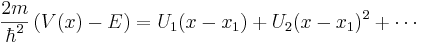
To first order, one finds
This differential equation is known as the Airy equation, and the solution may be written in terms of Airy functions.
![\Psi(x) = C_A \textrm{Ai}\left( \sqrt[3]{U_1} (x - x_1) \right) + C_B \textrm{Bi}\left( \sqrt[3]{U_1} (x - x_1) \right).](/2009-wikipedia_en_wp1-0.7_2009-05/I/1714a6dea70db9cbd0c6acaf0ec4fbd6.png)
This solution should connect the far away and beneath solutions. Given the 2 coefficients on one side of the classical turning point, the 2 coefficients on the other side of the classical turning point can be determined by using this local solution to connect them. Thus, a relationship between  and
and  can be found.
Fortunately the Airy functions will asymptote into sine, cosine and exponential functions in the proper limits. The relationship can be found to be as follows (often referred to as "connection formulas"):
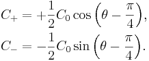
Now the global (approximate) solutions can be constructed.
Precision of the asymptotic series
The asymptotic series for  is usually a divergent series whose general term
  starts to increase after a certain value
  . Therefore the smallest error achieved by the WKB method is at best of the order of the last included term. For the equation
with  an analytic function, the value
  and the magnitude of the last term can be estimated as follows (see Winitzki 2005),
![\delta^{n_\max}S_{n_\max}(x_0) \approx \sqrt{\frac{2\pi}{n_\max}} \exp[-n_\max],](/2009-wikipedia_en_wp1-0.7_2009-05/I/ec7657b369c3ad6e6de133b52e3cfa9a.png)
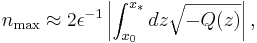
where  is the point at which
  needs to be evaluated and
  is the (complex) turning point where
  , closest to
  . The number can be interpreted as the number of oscillations between and the closest turning point. If
  is a slowly-changing function,
the number will be large, and the minimum error of the asymptotic series will be exponentially small.
See also
- Airy Function
- Langer correction
- Method of steepest descent / Laplace Method
- Perturbation methods
- Quantum tunneling
- Old quantum theory
References
Modern references
- Razavy, Moshen (2003). Quantum Theory of Tunneling. World Scientific. ISBN 981-238-019-1.
- Griffiths, David J. (2004). Introduction to Quantum Mechanics (2nd ed.). Prentice Hall. ISBN 0-13-111892-7.
- Liboff, Richard L. (2003). Introductory Quantum Mechanics (4th ed.). Addison-Wesley. ISBN 0-8053-8714-5.
- Sakurai, J. J. (1993). Modern Quantum Mechanics. Addison-Wesley. ISBN 0-201-53929-2.
- Bender, Carl; Orszag, Steven (1978). Advanced Mathematical Methods for Scientists and Engineers. McGraw-Hill. ISBN 0-07-004452-X.
- Olver, Frank J. W. (1974). Asymptotics and Special Functions. Academic Press. ISBN 0-12-525850-X.
- Winitzki, Sergei (2005). "Cosmological particle production and the precision of the WKB approximation". Physical Review D 72: 104011. doi:.
Historical references
- Carlini, Francesco (1817). Richerche sulla convergenza della serie che serva aal soluzione del problema di Keplero. Milano.
- Liouville, Joseph (1837). "Sur le développement des fonctions et séries..". Journal de Mathématiques Pures et Appliquées 1: 16–35.
- Green, George (1837). "On the motion of waves in a variable canal of small depth and width". Transactions of the Cambridge Philosophical Society 6: 457–462.
- Rayleigh, Lord (John William Strutt) (1912). "On the propagation of waves through a stratified medium, with special reference to the question of reflection". Proceedings of the Royal Society London, Series A 86: 207–226. doi:.
- Gans, Richard (1915). "Fortplantzung des Lichts durch ein inhomogenes Medium". Annalen der Physik 47: 709–736.
- Jeffreys, Harold (1924). "On certain approximate solutions of linear differential equations of the second order". Proceedings of the London Mathematical Society 23: 428–436. doi:.
- Brillouin, Léon (1926). "La mécanique ondulatoire de Schrödinger: une méthode générale de resolution par approximations successives". Comptes Rendus de l'Academie des Sciences 183: 24–26.
- Kramers, Hendrik A. (1926). "Wellenmechanik und halbzählige Quantisierung". Zeitschrift der Physik 39: 828–840. doi:.
- Wentzel, Gregor (1926). "Eine Verallgemeinerung der Quantenbedingungen für die Zwecke der Wellenmechanik". Zeitschrift der Physik 38: 518–529. doi:.
External links
- Richard Fitzpatrick, The W.K.B. Approximation (2002). (An application of the WKB approximation to the scattering of radio waves from the ionosphere.)
- Free WKB library for Microsoft Visual C v6 for some special functions