Vector space

In mathematics, a vector space is a collection of objects called vectors that may be scaled and added. These two operations must adhere to a number of axioms that generalize common properties of tuples of real numbers such as vectors in the plane or three-dimensional Euclidean space. Vector spaces are a keystone of linear algebra, and much of their theory is of a linear nature. From this viewpoint vector spaces are well-understood, since they are completely specified by a single number called dimension.
Historically, the first ideas leading to modern vector spaces can be traced as far as 17th century's analytic geometry, matrices and systems of linear equations. The modern, axiomatic treatment was first formulated by Giuseppe Peano, in the late 19th century. Later enhancements of the theory are due to the widespread presence of vector spaces in mathematical analysis, mainly in the guise of function spaces. Analytical problems call for a notion that goes beyond linear algebra by taking into account convergence questions. This is done by considering vector spaces with additional data, mostly spaces endowed with a suitable topology, thus allowing to take into account proximity and continuity issues. These topological vector spaces, in particular Banach spaces and Hilbert spaces have a richer and more complicated theory.
Vector spaces are applied throughout mathematics, science and engineering. They are used in methods such as Fourier expansion, which is used in modern sound and image compression routines, or provides the framework to solution techniques of partial differential equations. Furthermore, vector spaces furnish an abstract, coordinate-free way of dealing with geometrical and physical objects such as tensors, which in turn allows to examine local properties of manifolds by linearization techniques.
Contents |
Motivation and definition

The space R2, consisting of pairs (x, y) of real numbers, is a common example of a vector space: any two pairs of real numbers can be added,
- (x1, y1) + (x2, y2) = (x1 + x2, y1 + y2),
and any pair (x, y) can be multiplied by a real number s to yield another vector (sx, sy).
The notion of a vector space is an extension of this idea, and is more general in several ways. Firstly, instead of the real numbers other fields, such as the complex numbers or finite fields, are allowed.[nb 1] Secondly, the dimension of the space (which is two in the above example) can be an arbitrary non-negative integer or infinite. Another conceptually important point is that elements of vector spaces are not usually expressed as linear combinations of a particular set of vectors, i.e., there is no preference of representing the vector (x, y) as
-
- (x, y) = x · (1, 0) + y · (0, 1)
- over
- (x, y) = (−1/3·x + 2/3·y) · (−1, 1) + (1/3·x + 1/3·y) · (2, 1)
Definition
The definition of a vector space requires a field F such as the field of rational, real or complex numbers. A vector space is a set V together with two operations that combine two elements to a third:
- vector addition: any two vectors, i.e. elements of V, v and w can be added to yield a third vector v + w
- scalar multiplication: any vector v can be multiplied by a scalar, i.e. element of F, a. The product is denoted av.
To specify the field F, one speaks of F-vector space, vector space over F. For F = R or C, they are also called real and complex vector spaces, respectively. To qualify as a vector space, the addition and multiplication have to adhere to a number of requirements called axioms generalizing the situation of Euclidean plane R2 or Euclidean space R3.[1] For distinction, vectors v will be denoted in boldface.[nb 2] In the formulation of the axioms below, let u, v, w be arbitrary vectors in V, and a, b be scalars, respectively.
| Axiom | Signification |
| Associativity of addition | u + (v + w) = (u + v) + w |
| Commutativity of addition | v + w = w + v |
| Identity element of addition | There exists an element 0 ∈ V, called the zero vector, such that v + 0 = v for all v ∈ V. |
| Inverse elements of addition | For all v ∈ V, there exists an element w ∈ V, called the additive inverse of v, such that v + w = 0. |
| Distributivity of scalar multiplication with respect to vector addition | a (v + w) = a v + a w |
| Distributivity of scalar multiplication with respect to field addition | (a + b) v = a v + b v |
| Compatibility of scalar multiplication with field multiplication | a (b v) = (ab) v [nb 3] |
| Identity element of scalar multiplication | 1 v = v, where 1 denotes the multiplicative identity in F |
The space V = R2 over the real numbers, with the addition and multiplication as above, is indeed a vector space. Checking the axioms reduces to verifying simple identities such as
- (x, y) + (0, 0) = (x, y),
i.e. the addition of the zero vector (0, 0) to any other vector yields that same vector. The distributive law amounts to
- (a + b) · (x, y) = a · (x, y) + b · (x, y).
Alternative formulations and elementary consequences of the definition
The requirement that vector addition and scalar multiplication be binary operations includes (by definition of binary operations) a property called closure, i.e. u + v and a v are in V for all a, u, and v. Some authors choose to mention these properties as separate axioms.
The first four axioms can be subsumed by requiring the set of vectors to be an abelian group under addition, and the rest are equivalent to a ring homomorphism f from the field into the endomorphism ring of the group of vectors. Then scalar multiplication a v is defined as (f(a))(v). This can be seen as the starting point of defining vector spaces without referring to a field.[2]
There are a number of properties that follow easily from the vector space axioms. Some of them derive from elementary group theory, applied to the (additive) group of vectors: for example the zero vector 0 ∈ V and the additive inverse −v of a vector v are unique. Other properties can be derived from the distributive law, for example scalar multiplication by zero yields the zero vector and no other scalar multiplication yields the zero vector.
History
- Further information: History of algebra
Vector spaces stem from affine geometry, via the introduction of coordinates in the plane or three-dimensional space. Around 1636, French mathematicians Descartes and Fermat founded the bases of analytic geometry by tying the solutions of an equation with two variables to the determination of a plane curve.[3] To achieve a geometric solutions without using coordinates, Bernhard Bolzano introduced in 1804 certain operations on points, lines and planes, which are predecessors of vectors.[4] This work was made use of in the conception of barycentric coordinates of August Ferdinand Möbius in 1827.[5] The founding leg of the definition of vectors was the Bellavitis' definition of the bipoint, which is an oriented segment, one of whose ends is the origin and the other one a target. Vectors were reconsidered with the presentation of complex numbers by Argand and Hamilton and the inception of quaternions by the latter.[6] They are elements in R2 and R4; treating them using linear combinations goes back to Laguerre in 1867, who also defined systems of linear equations.
In 1857, Cayley introduced the matrix notation which allows for a harmonization and simplification of linear maps. Around the same time, Grassmann studied the barycentric calculus initiated by Möbius. He envisaged sets of abstract objects endowed with operations.[7] In his work, the concepts of linear independence and dimension, as well as scalar products are present. Actually Grassmann's 1844 work exceeds the framework of vector spaces, since his considering multiplication, too, led him to what is today are called algebras. Italian mathematician Peano first gave the modern definition of vector spaces and linear maps in 1888.[8]
An important development of vector spaces is due to the construction of function spaces by Henri Lebesgue. This was later formalized by Banach's 1920 PhD thesis and Hilbert.[9] At this time, algebra and the new field of functional analysis began to interact, notably with key concepts such as spaces of p-integrable functions and Hilbert spaces. Also at this time, the first studies concerning infinite-dimensional vector spaces were done.
Examples
Coordinate and function spaces
The first example of a vector space over a field F is the field itself, equipped with its standard addition and multiplication. This is generalized by the vector space known as the coordinate space and usually denoted Fn, where n is an integer. Its elements are n-tuples
- (a1, a2, ..., an), where the ai are elements of F.[10]
Infinite coordinate sequences, and more generally functions from any fixed set Ω to a field F also form vector spaces, by performing addition and scalar multiplication pointwise, i.e. the sum of two functions f and g is given by
- (f + g)(w) = f(w) + g(w)
and similarly for multiplication. Such function spaces occur in many geometric situations, when Ω is the real line or an interval, or other subsets of Rn. Many notions in topology and analysis, such as continuity, integrability or differentiability are well-behaved with respect to linearity, i.e. sums and scalar multiples of functions possessing such a property will still have that property.[11] Therefore, the set of such functions are vector spaces. They are studied in more detail using the methods of functional analysis, see below. Algebraic constraints also yield vector spaces: the vector space F[x] is given by polynomial functions, i.e.
- f (x) = rnxn + rn−1xn−1 + ... + r1x + r0, where the coefficients rn, ..., r0 are in F.[12]
Power series are similar, except that infinitely many terms are allowed.[13]
Linear equations
Systems of homogeneous linear equations are closely tied to vector spaces.[14] For example, the solutions of
-
a + 3b + c = 0 4a + 2b + 2c = 0
are given by triples with arbitrary a, b = a/2, and c = −5a/2. They form a vector space: sums and scalar multiples of such triples still satisfy the same ratios of the three variables; thus they are solutions, too. Matrices can be used to condense multiple linear equations as above into one vector equation, namely
- Ax = 0,
where A is the matrix
 ,
,
x is the vector (a, b, c), and 0 = (0, 0) is the zero vector. In a similar vein, the solutions of homogeneous linear differential equations form vector spaces. For example
- f ''(x) + 2f '(x) + f (x) = 0
yields f (x) = a · e−x + bx · e−x, where a and b are arbitrary constants, and e = 2.718....
Field extensions
A common situation in algebra, and especially in algebraic number theory is a field F containing a smaller field E. By the given multiplication and addition operations of F, F becomes an E-vector space, also called a field extension of E.[15] For example the complex numbers are a vector space over R. Another example is Q(z), the smallest field containing the rationals and some complex number z.
Bases and dimension
Bases reveal the structure of vector spaces in a concise way. Intuitively, a base for a vector space generates the vector space (just as a basis for a topology generates a topology or a generator in group theory generates the group it belongs to). Formally, a basis is a (finite or infinite) set B = {vi}i ∈ I of vectors that spans the whole space, and minimal with this property. The former means that any vector v can be expressed as a finite sum (called linear combination) of the basis elements
- a1vi1 + a2vi2 + ... + anvin,
where the ak are scalars and vik (k = 1, ..., n) elements of the basis B. The minimality, on the other hand, is made formal by the notion of linear independence. A set of vectors is said to be linearly independent if none of its elements can be expressed as a linear combination of the remaining ones. Equivalently, an equation
- a1vi1 + ai2v2 + ... + anvin = 0
can only hold if and only if all scalars a1, ..., an equal zero. By definition every vector can be expressed as a finite sum of basis elements. Because of linear independence any such representation is unique.[16] Vector spaces are sometimes introduced from this coordinatised viewpoint.
Every vector space has a basis. This fact relies on Zorn’s Lemma, an equivalent formulation of the axiom of choice.[17] Given the other axioms of Zermelo-Fraenkel set theory, the existence of bases is equivalent to the axiom of choice.[18] The ultrafilter lemma, which is weaker than the axiom of choice, implies that all bases of a given vector space have the same "size", i.e. cardinality.[19] It is called the dimension of the vector space, denoted dim V. If the space is spanned by finitely many vectors, the above statements can be proven without such fundamental input from set theory.[20]
The dimension of the coordinate space Fn is n, since any vector (x1, x2, ..., xn) can be uniquely expressed as a linear combination of n vectors (called coordinate vectors) e1 = (1, 0, ..., 0), e2 = (0, 1, 0, ..., 0), to en = (0, 0, ..., 0, 1), namely the sum
- x1e1 + x2e2 + ... + xnen,
The dimension of function spaces, such as the space of functions on some bounded or unbounded interval, is infinite.[nb 4] Under suitable regularity assumptions on the coefficients involved, the dimension of the solution space of an homogeneous ordinary differential equation equals the degree of the equation.[21] For example, the above equation has degree 2. The solution space is generated by ex and xex (which are linearly independent over R), so the dimension of this space is two.
The dimension (or degree) of a field extension such as Q(z) over Q depends on whether or not z is algebraic, i.e. satisfies some polynomial equation
- qnzn + qn−1zn−1 + ... + q0 = 0, with rational coefficients qn, ..., q0.
If it is algebraic the dimension is finite. More precisely, it equals the degree of the minimal polynomial having this number as a root.[22] For example, the complex numbers are a two-dimensional real vector space, generated by 1 and the imaginary unit i. The latter satisfies i2 + 1 = 0, an equation of degree two. Likewise, C is a two-dimensional R-vector space (and, as any field, one-dimensional as a vector space over itself, C). If z is not algebraic, the degree of Q(z) over Q is infinite. For instance, for z = π there is no such equation, since π is transcendental.[23]
Linear maps and matrices
As with many algebraic entities, the relation of two vector spaces is expressed by maps between them. In the context of vector spaces, the corresponding concept is called linear maps or linear transformations.[24] They are functions f : V → W that are compatible with the relevant structure—i.e., they preserve sums and scalar multiplication:
- f(v + w) = f(v) + f(w) and f(a · v) = a · f(v).
An isomorphism is a linear map f : V → W such that there exists an inverse map g : W → V, i.e. a map such that the two possible compositions f ∘ g : W → W and g ∘ f : V → V are identity maps. Equivalently, f is both one-to-one (injective) and onto (surjective).[25] If there exists an isomorphism between V and W, the two spaces are said to be isomorphic; they are then essentially identical as vector spaces, since all identities holding in V are, via f, transported to similar ones in W, and vice versa via g.
Given any two vector spaces V and W, linear maps V → W form a vector space HomF(V, W), also denoted L(V, W).[26] The space of linear maps from V to F is called the dual vector space, denoted V∗.[27]
Once a basis of V is chosen, linear maps f : V → W are completely determined by specifying the images of the basis vectors, because any element of V is expressed uniquely as a linear combination of them.[28] If dim V = dim W, one can choose a 1-to-1 correspondence between two fixed bases of V and W. The map that maps any basis element of V to the corresponding basis element of W is, by its very definition, an isomorphism.[29] Thus any vector spaces is completely classified (up to isomorphism) by its dimension, a single number. In particular, any n-dimensional vector spaces over F is isomorphic to Fn. Hence, there are only countably many isomorphism classes of vector spaces over a fixed field.
Matrices

Matrices are a useful notion to encode linear maps.[30] They are written as a rectangular array of scalars, i.e. elements of some field F. Any m-by-n matrix A gives rise to a linear map from Fn to Fm, by the following
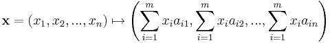 ,
,
or, using the matrix multiplication of the matrix A with the coordinate vector x:
- x ↦ Ax.
Moreover, after choosing bases of V and W, any linear map f : V → W is uniquely represented by a matrix via this assignment.[31]

The determinant det (A) of a square matrix A is a scalar that tells whether the associated map is an isomorphism or not: to be so it is sufficient and necessary that the determinant is nonzero.[32] The determinant of a real square matrix also determines whether the corresponding linear transformation is orientation preserving or not: it is so if and only if the determinant is positive.
Eigenvalues and eigenvectors
A particularly important case are endomorphisms, i.e. maps f : V → V. In this case, vectors v can be compared to their image under f, f(v). Any nonzero vector v satisfying λ · v = f(v), where λ is a scalar, is called an eigenvector of f with eigenvalue λ.[nb 5][33] The set of all eigenvectors corresponding to a particular eigenvalue (and a particular f) forms a vector space known as the eigenspace corresponding to the eigenvalue (and f) in question. Equivalently, v is an element of kernel of the difference f − λ · Id (the identity map V → V). In the finite-dimensional case, this can be rephrased using determinants: f having eigenvalue λ is the same as
- det (f − λ · Id) = 0.
By spelling out the definition of the determinant, the expression on the left hand side turns out to be a polynomial function in λ, called the characteristic polynomial of f.[34] If the field F is large enough to contain a zero of this polynomial (which automatically happens for F algebraically closed, such as F = C) any linear map has at least one eigenvector. The vector space V may or may not possess an eigenbasis, i.e. a basis consisting of eigenvectors. This phenomenon is governed by the Jordan canonical form of the map.[nb 6] The spectral theorem describes the infinite-dimensional case; to accomplish this aim, the machinery of functional analysis is needed, see below.
Basic constructions
In addition to the above concrete examples, there are a number of standard linear algebraic constructions that yield vector spaces related to given ones. In addition to the concrete definitions given below, they are also characterized by universal properties, which determines an object X by specifying the linear maps from X to any other vector space.[35]
Subspaces and quotient spaces

In general, a nonempty subset W of a vector space V that is closed under addition and scalar multiplication is called a subspace of V.[36] Subspaces of V are vector spaces (over the same field) in their own right. The intersection of all subspaces containing a given set S of vectors is called its span. Expressed in terms of elements, the span is the subspace consisting linear combinations of elements of S.[37]
The counterpart to subspaces are quotient vector spaces.[38] Given any subspace W ⊂ V, the quotient space V/W ("V modulo W") is defined as follows: as a set, it consists of v + W = {v + w, w ∈ W}, where v is an arbitrary vector in V. The sum of two such elements v1 + W and v2 + W is (v1 + v2) + W, and scalar multiplication is given by a · (v + W) = (a · v) + W. The key point in this definition is that v1 + W = v2 + W if and only if the difference of v1 and v2 lies in W.[nb 7] This way, the quotient space "forgets" information that is contained in the subspace W.
For any linear map f : V → W, the kernel ker(f ) consists of vectors v that are mapped to 0 in W.[39] Both kernel and image im(f ) = {f(v), v ∈ V}, are linear subspaces of V and W, respectively.[40] They are related by an elementary but fundamental isomorphism
- V / ker(f ) ≅ im(f ).
The existence of kernels and images is part of the statement that the category of vector spaces (over a fixed field F) is an abelian category.[41]
An important example is the kernel of a linear map x ↦ Ax for some fixed matrix A, as above. The kernel of this map, i.e. the subspace of vectors x such that Ax = 0 are precisely the solutions to the system of linear equations belonging to A. This concept also comprises linear differential equations
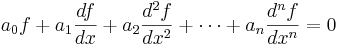 , where the coefficients ai are functions in x, too.
In the corresponding map
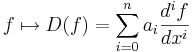 ,
,
the derivatives of the function f appear linearly (as opposed to f ''(x)2, for example). Since differentiation is a linear procedure (i.e. (f + g)' = f ' + g ' and (c·f)' = c·f ' for a constant c) this assignment is linear, called a linear differential operator. In particular, the solutions to the differential equation D(f ) = 0 form a vector space (over R or C).
Direct product and direct sum
The direct product  of a family of vector spaces Vi, where i runs through some index set I, consists of tuples (vi)i ∈ I, i.e. for any index i, one element vi of Vi is given.[42] Addition and scalar multiplication is performed componentwise. A variant of this construction is the direct sum
  (also called coproduct and denoted
  ), where only tuples with finitely many nonzero vectors are allowed. If the index set I is finite, the two constructions agree, but differ otherwise.
Tensor product
The tensor product V ⊗F W, or simply V ⊗ W is one of the central notions of multilinear algebra. It is a vector space consisting of finite (formal) sums of symbols
- v1 ⊗ w1 + v2 ⊗ w2 + ... + vn ⊗ wn,
subject to certain rules mimicking bilinearity, such as
- a · (v ⊗ w) = (a · v) ⊗ w = v ⊗ (a · w).[43]
Via the fundamental adjunction isomorphism (for finite-dimensional V and W)
- HomF (V, W) ≅ V∗ ⊗F W [44]
matrices, which are essentially the same as linear maps, i.e. contained in the left hand side, translate into an element of the tensor product of the dual of V with W. Therefore the tensor product may be seen as the extension of the hierarchy of scalars, vectors and matrices.
Vector spaces with additional structure
From the point of view of linear algebra, vector spaces are completely understood insofar as any vector space is characterized, up to isomorphism, by its dimension. However, vector spaces ad hoc do not offer a framework to deal with the question—crucial to analysis—whether a sequence of functions converges to another function. Likewise, linear algebra is not per se adapted to deal with infinite series, since the addition operation allows only finitely many terms to be added. The needs of functional analysis require considering additional structures. Much the same way the formal treatment of vector spaces reveals their essential algebraic features, studying vector spaces with additional datums abstractly turns out to be advantageous, too.
A first example of an additional datum is an order ≤, a token by which vectors can be compared.[45] Rn can be ordered by comparing the vectors componentwise. Ordered vector spaces, for example Riesz spaces, are basal to Lebesgue integration, which stakes on expressing a function as a difference of two positive functions
- f = f + − f −,
i.e. the positive f + and negative part f −, respectively.[46]
Normed vector spaces and inner product spaces
"Measuring" vectors is a frequent need, either by specifying a norm, a datum which measures the lengths of vectors, or by an inner product, which measures the angles between vectors. The latter entails that lengths of vectors can be defined too, by defining the associated norm 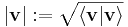 . Vector spaces endowed with such data are known as normed vector spaces and inner product spaces, respectively.[47]
Coordinate space Fn can be equipped with the standard dot product:
- 〈x | y〉 = x · y = x1y1 + ... + xnyn.
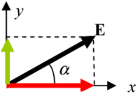
In R2, this reflects the common notion of the angle between two vectors x and y, by the law of cosines:

Because of this, two vectors satisfying 〈x | y〉 = 0 are called orthogonal.
An important variant of the standard dot product is used in Minkowski space, i.e. R4 endowed with the inner product
- 〈x | y〉 = x1y1 + x2y2 + x3y3 − x4y4.[48]
It is crucial to the mathematical treatment of special relativity, where the fourth coordinate—corresponding to time, as opposed to three space-dimensions—is singled out.
Topological vector spaces

 .
.Convergence questions are addressed by considering vector spaces V carrying a compatible topology, i.e. a structure that allows to talk about elements being close to each other.[49][50] Compatible here means that addition and scalar multiplication should be continuous maps, i.e. if x and y in V, and a in F vary by a bounded amount, then so do x + y and ax.[nb 8] To make sense of specifying the amount a scalar changes, the field F also has to carry a topology in this setting; a common choice are the reals or the complex numbers.
In such topological vector spaces one can consider infinite sums of vectors, i.e. series, by writing

for the limit of the corresponding finite sums of functions. For example, the fi could be (real or complex) functions, and the limit takes place in some function space. The type of convergence obtained depends on the used topology. Pointwise convergence and absolute convergence are two prominent examples.
A way of ensuring the existence of limits of such infinite series is to restrict attention to spaces where any Cauchy sequence has a limit, i.e. complete vector spaces. Roughly, completeness means the absence of holes. For example, the rationals are not complete, since there are series of rational numbers converging to irrational numbers such as .[51] Banach and Hilbert spaces, are complete topological spaces whose topology is given by a norm and an inner product, respectively. Their study is a key piece of functional analysis. The theory focusses on infinite-dimensional vector spaces, since all norms on finite-dimensional topological vector spaces are equivalent, i.e. give rise to the same notion of convergence.[52] The image at the right shows the equivalence of the 1-norm and ∞-norm on R2: as the unit "balls" enclose each other, a sequence converges to zero in one norm if and only if it so does in the other norm. In the infinite-dimensional case, however, there will generally be inequivalent topologies, which makes the study of topological vector spaces richer than that of vector spaces without additional data.
From a conceptual point of view, all notions related to topological vector spaces should match the topology. For example, instead of considering all linear maps (also called functionals) V → W, it is useful to require maps to be continuous.[53] For example, the dual space V∗ consists of continuous functionals V → R (or C). Applying the dual construction twice yields the bidual V∗∗. The natural map V → V∗∗ is always injective, thanks to the fundamental Hahn-Banach theorem.[54] If it is an isomorphism, V is called reflexive.
Banach spaces
Banach spaces, introduced by Stefan Banach, are complete normed vector spaces.[55] A first example is the vector space lp consisting of infinite vectors with real entries x = (x1, x2, ...) whose p-norm (1 ≤ p ≤ ∞) given by
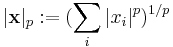 for p < ∞ and
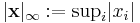
is finite. The topologies on the infinite-dimensional space lp are inequivalent for different p. E.g. the sequence of vectors xn = (2−n, 2−n, ..., 2−n, 0, 0, ...), i.e. the first 2n components are 2−n, the following ones are 0, converges to the zero vector for p = ∞, but does not for p = 1:
 , but
, but  .
.
More generally, functions f : Ω → R are endowed with a norm that replaces the above sum by the Lebesgue integral
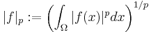 .
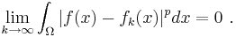
.The space of integrable functions on a given domain Ω (for example an interval) satisfying |f |p < ∞, and equipped with this norm are called Lebesgue spaces, denoted Lp(Ω). These spaces are complete.[56] (If one uses the Riemann integral instead, the space is not complete, which may be seen as a justification for Lebesgue's integration theory.[nb 10]) Concretely this means that for any sequence of Lebesgue-integrable functions f1(x), f2(x), ... with |fn|p < ∞, satisfying the condition
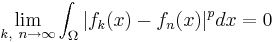
there exists a function f(x) belonging to the vector space Lp(Ω) such that
Imposing boundedness conditions not only on the function, but also on its derivatives leads to Sobolev spaces.[57]
Hilbert spaces

Complete inner product spaces are known as Hilbert spaces, in honor of David Hilbert.[58] A key case is the Hilbert space L2(Ω), with inner product given by
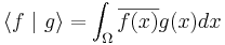 , with
  being the complex conjugate of f(x).
By definition, Cauchy sequences in any Hilbert space converge, i.e. have a limit. Conversely, finding a sequence of functions fn with desirable properties that approximates a given limit function, is equally crucial. Early analysis, in the guise of the Taylor approximation, established an approximation of differentiable functions f by polynomials.[61] By the Stone-Weierstrass theorem, every continuous function on [a, b] can be approximated as closely as desired by a polynomial.[62] More generally, and more conceptually, the theorem yields a simple description of what "basic functions" suffice to generate a Hilbert space H, in the sense that the closure of their span (i.e. finite linear combinations and limits of those) is the whole space. Such a set of functions is called a Hilbert basis of H, its cardinality is known as the Hilbert dimension.[nb 11] Not only does the theorem exhibit suitable basis functions as sufficient for approximation purposes, together with the Gram-Schmidt process, it also allows to construct a basis of orthogonal vectors.[63] Ortoghonal bases are the Hilbert space generalization of the coordinate axes in (finite-dimensional) Euclidean space. A similar approximation technique by trigonometric functions is commonly called Fourier expansion, and is much applied in engineering, see below.
The solutions to various important differential equations can be interpreted in terms of Hilbert spaces. For example, a great many fields in physics and engineering lead to such equations and frequently solutions with particular physical properties are used as basis functions, often orthogonal, that serve as the axes in a corresponding Hilbert space.[64] As an example from physics, the time-dependent Schrödinger equation in quantum mechanics describes the change of physical properties in time, by means of a partial differential equation determining a wavefunction.[65] Definite values for physical properties such as energy, or momentum, correspond to eigenvalues of a certain (linear) differential operator and the associated wavefunctions are called eigenstates. The spectral theorem decomposes a linear compact operator that acts upon functions in terms of these eigenfunctions and their eigenvalues.[66]
Algebras over fields

In general, vector spaces do not possess a multiplication operation. A vector space equipped with an additional bilinear operator defining the multiplication of two vectors is an algebra over a field.[67] Many algebras stem from functions on some geometrical object: since functions with values in a field can be multiplied, these entities form algebras. The Stone-Weierstrass theorem mentioned above, for example, relies on Banach algebras which are at the junction of Banach spaces and algebras.
Commutative algebra makes great use of rings of polynomials in one or several variables, introduced above, where multiplication is both commutative and associative. These rings and their quotients form the basis of algebraic geometry, because they are rings of functions of algebraic geometric objects.[68]
Another crucial example are Lie algebras, which are neither commutative, nor associative, but the failure to be so is limited by the constraints ([x, y] denotes the product of x and y):
- anticommutativity [x, y] = −[y, x] and the Jacobi identity [x, [y, z]] + [y, [x, z]] + [z, [x, y]] = 0.[69]
The standard example is the vector space of n-by-n matrices, with [x, y] = xy − yx, the commutator of two matrices. Another example is R3, endowed with the cross product.
A formal way of adding products to any vector space V, i.e. obtaining an algebra, is to produce the tensor algebra T(V).[70] It is built of symbols, called tensors
- v1 ⊗ v2 ⊗ ... ⊗ vn, where the rank n varies.
The multiplication is given by concatenating two such symbols. In general, there are no relations between v1 ⊗ v2 and v2 ⊗ v1. Forcing two such elements to be equal leads to the symmetric algebra, whereas forcing v1 ⊗ v2 = − v2 ⊗ v1 yields the exterior algebra.[71]
Applications
Vector spaces occur in many mathematical circumstances, namely whenever functions (with values in some field) are involved, there are manifold applications: they provide a framework to deal with analytical and geometrical problems, or are used in the Fourier transform. This list is not exhaustive: many more applications exist, for example in optimization.[72]
Distributions
A distribution (or generalized function) is a linear map assigning a number to "test" functions f, i.e. smooth functions with compact support, in a continuous way, i.e. in the above terminology they are just elements of the (continuous) dual of the test function space.[73] The latter space is endowed with a topology that takes into account not only f itself, but also all its higher derivatives. Two standard examples are given by integrating the test function f over some domain Ω, and the Dirac distribution:
 and
and 
Distributions are a powerful instrument to solve differential equations. Since all standard analytic notions such as derivatives are linear, they extend naturally to the space of distributions. Therefore the equation in question can be transferred to a distribution space, which are strictly bigger than the underlying function space, so more flexible methods, for example using Green's functions (which usually aren't functions, but distributions) can be used to find a solution. The found solution can then in some cases be proven to be actually a true function, and a solution to the original equation (e.g. using the Lax-Milgram theorem, a consequence of the Riesz representation theorem).[74]
Fourier expansion
Resolving a periodic function f(x) into sums of trigonometric functions is known as the Fourier expansion, a technique much used in physics and engineering.[75] By the Stone-Weierstrass theorem (see above), any function f(x) on a bounded, closed interval (or equivalently, any periodic function) is a limit of functions of the following type
![f_N (x) = \frac{a_0}{2} + \sum_{m=1}^{N}\left[a_m\cos\left(mx\right)+b_m\sin\left(mx\right)\right]](/2009-wikipedia_en_wp1-0.7_2009-05/I/481f2565f4430bf5329d95b2b6738a48.png)
as N → ∞ . The coefficients am and bm are called Fourier coefficients of f.
The historical motivation to this were differential equations: Fourier, in 1822, used the technique to give the first solution of the heat equation.[76] Other than that, the discrete Fourier transform is used in jpeg image compression[77] or, in the guise of Fast Fourier Transform, for high-speed multiplications of large integers.[78]
Geometry

The tangent space TxM of a differentiable manifold M (for example a smooth curve in Rn such as a circle) at a point x of M is a way to flatten or "linearize" the manifold at that point.[79] It may reveal a great deal of information about the manifold: the tangent space of Lie groups is natuarlly a Lie algebra and can be used to classify compact Lie groups.[80] Getting back from the tangent space to the manifold is accomplished by the vector flow.
The dual of the tangent space is called cotangent space. Differential forms are elements of the exterior algebra of the cotangent space. They generalize the "dx" in standard integration
 .
.
Further vector space constructions, in particular tensors are widely used in geometry and beyond. Riemannian manifolds are manifolds whose tangent spaces are endowed with a suitable inner product.[81] Derived therefrom, the Riemann curvature tensor encodes all curvatures of a manifold in one object, which finds applications in general relativity, for example, where the Einstein curvature tensor describes the curvature of space-time.[82][83]
The cotangent space is also used in commutative algebra and algebraic geometry to define regular local rings, an algebraic adaptation of smoothness in differential geometry, by comparing the dimension of the cotangent space of the ring (defined in a purely algebraic manner) to the Krull dimension of the ring.[84]
Generalizations
Vector bundles

A family of vector spaces, parametrised continuously (resp. smoothly) by some topological space (resp. differentiable manifold) X, is a vector bundle (resp. smooth vector bundle).[85] More precisely, a vector bundle E over X is given by a continuous map
- π : E → X,
which is locally a product of X with some (fixed) vector space V, i.e. such that for every point x in X, there is a neighborhood U of x such that the restriction of π to π−1(U) equals the projection V × U → U (the "trivialization" of the bundle over U).[nb 12] The case dim V = 1 is called a line bundle. While the situation is simple to oversee locally, there may be—depending on the shape of the underlying space X—global twisting phenomena. For example, the Möbius strip can be seen as a line bundle over the circle S1 (at least if one extends the bounded interval to infinity). The (non-)existence of vector bundles with certain properties can tell something about the underlying topological space. By the hairy ball theorem, for example, there is no tangent vector field on the 2-sphere S2 which is everywhere nonzero, in contrast to the circle S1, whose tangent bundle (i.e. the bundle consisting of the tangent spaces TxM at all points x of M) is trivial, i.e. globally isomorphic to S1 × R [86]. K-theory studies the ensemble of all vector bundles over some topological space.[87]
Modules
Modules are to rings what vector spaces are to fields, i.e. the very same axioms, applied to a ring R instead of a field F yield modules.[88] In contrast to the exhaustive understanding of vector spaces offered by linear algebra, the theory of modules is much more complicated, because of ring elements that do not possess multiplicative inverses. For example, modules need not have bases as the Z-module (i.e. abelian group) Z/2 shows; those modules that do (including all vector spaces) are known as free modules. The algebro-geometric interpretation of commutative rings via their spectrum allows to develop concepts such as locally free modules, which are the algebraic counterpart to vector bundles. In the guise of projective modules they are important in homological algebra[89] and algebraic K-theory.[90]
Affine and projective spaces

Roughly, affine spaces are vector spaces whose origin is not specified.[91] More precisely, an affine space is a set with a transitive vector space action. In particular, a vector space is an affine space over itself, by the map
- V2 → V, (a, b) ↦ a − b.
Sets of the form x + V (viewed as a subset of some bigger space W), i.e. translating some linear subspace V by a fixed vector x yields affine spaces, too. In particular, this notion encloses all solution of systems of linear equations
- Ax = b
generalizing the homogenouos case (i.e. b = 0) above.[92]
The set of one-dimensional subspaces of a fixed finite-dimensional vector space V is known as projective space, an important geometric object formalizing the idea of parallel lines intersecting at infinity.[93] More generally, the Grassmannian manifold consists of linear subspaces of higher (fixed) dimension n. Finally, flag manifolds parametrize flags, i.e. chains of subspaces (with fixed dimension)
- 0 = V0 ⊂ V1 ⊂ ... ⊂ Vn = V.
See also
- Clifford algebra
- Coordinates (mathematics)
- Covariant derivative
- Differentiable manifold
- Graded vector space
- Euclidean vector, for vectors in physics
- Immersion
- Lie derivative
- P-vector
- Riesz-Fischer theorem
- Submersion
Notes
- ↑ Some authors (such as Brown 1991) restrict attention to the fields R or C, but most of the theory is unchanged over an arbitrary field.
- ↑ It is also common, especially in physics, to denote vectors with an arrow on top:
 .
. - ↑ This axiom is not asserting the associativity of an operation, since there are two operations in question, scalar multiplication: b v; and field multiplication: ab.
- ↑ The indicator functions of intervals (of which there are infintely many) are linearly independent, for example.
- ↑ . The nomenclature derives from German "eigen", which means own or proper.
- ↑ Roman 2005, ch. 8, p. 140. See also Jordan–Chevalley decomposition
- ↑ Some authors (such as Roman 2005) choose to start with this equivalence relation and derive the concrete shape of V/W from this.
- ↑ This requirement implies that the topology gives rise to a uniform structure, Bourbaki 1989, ch. II
- ↑ The triangle inequality for |−|p is provided by the Minkowski inequality. For technical reasons, in the context of functions one has to identify functions that agree almost everywhere to get a norm, and not only a seminorm.
- ↑ "Many functions in L2 of Lebesgue measure, being unbounded, cannot be integrated with the classical Riemann integral. So spaces of Riemann integrable functions would not be complete in the L2 norm, and the orthogonal decomposition would not apply to them. This shows one of the advantages of Lebesgue integration.", Dudley 1989, sect. 5.3, p. 125.
- ↑ Sometimes, Hilbert bases are simply called bases. For distinction, a basis in the linear algebraic sense as above is then called a Hamel basis
- ↑ Additionally, the transition maps between two such trivializations are required to be linear maps on V.
Citations
- ↑ Roman 2005, ch. 1, p. 27.
- ↑ Ricci 2008.
- ↑ Bourbaki 1969, ch. "Algèbre linéaire et algèbre multilinéaire", pp. 78–91.
- ↑ Bolzano 1804.
- ↑ Möbius 1827.
- ↑ Hamilton 1853.
- ↑ Grassmann 2000.
- ↑ Peano 1888, ch. IX.
- ↑ Banach 1922.
- ↑ Lang 1987, ch. I.1
- ↑ e.g. Lang 1993, ch. XII.3., p. 335
- ↑ Lang 1987, ch. IX.1
- ↑ Lang 2002, ch. IV.9
- ↑ Lang 1987, ch. VI.3.
- ↑ Lang 2002, ch. V.1
- ↑ Lang 1987, ch. II.2., pp. 47–48
- ↑ Roman 2005, Theorem 1.10, p. 37.
- ↑ Blass 1984.
- ↑ Halpern 1966, pp. 670–673.
- ↑ Artin 1991, Theorem 3.3.13.
- ↑ Braun 1993, Th. 3.4.5, p. 291.
- ↑ Stewart 1975, Proposition 4.3, p. 52.
- ↑ Stewart 1975, Theorem 6.5, p. 74.
- ↑ Roman 2005, ch. 2, p. 45.
- ↑ Lang 1987, ch. IV.4, Corollary, p. 106.
- ↑ Lang 1987, Example IV.2.6.
- ↑ Lang 1987, ch. VI.6.
- ↑ Lang 1987, Theorem IV.2.1, p. 95.
- ↑ Roman 2005, Th. 2.5 and 2.6, p. 49.
- ↑ Lang 1987, ch. V.1.
- ↑ Lang 1987, ch. V.3., Corollary, p. 106.
- ↑ Lang 1987, Theorem VII.9.8, p. 198.
- ↑ Roman 2005, ch. 8, p. 135–156.
- ↑ Lang 1987, ch. IX.4.
- ↑ See Roman 2005, Th. 14.3 for the universal property of the tensor product. See also Yoneda lemma.
- ↑ Roman 2005, ch. 1, p. 29.
- ↑ Roman 2005, ch. 1, p. 35.
- ↑ Roman 2005, ch. 3, p. 64.
- ↑ Lang 1987, ch. IV.3..
- ↑ Roman 2005, ch. 2, p. 48.
- ↑ Mac Lane 1998.
- ↑ Roman 2005, ch. 1, p. 31–32.
- ↑ Lang 2002, ch. XVI.1
- ↑ Lang 2002, Cor. XVI.5.5
- ↑ Schaefer & Wolff 1999, pp. 204–205
- ↑ Bourbaki 2004, ch. 2, p. 48.
- ↑ Roman 2005, ch. 9.
- ↑ Naber 2003, ch. 1.2.
- ↑ Treves 1967.
- ↑ Bourbaki 1987.
- ↑ Goldrei 1996, Margin note of Th. 2.2, p. 13
- ↑ Choquet 1966, Proposition III.7.2.
- ↑ Treves 1967, p. 34–36.
- ↑ Lang 1983, Cor. 4.1.2, p. 69.
- ↑ Treves 1967, ch. 11.
- ↑ Treves 1967, Theorem 11.2, p. 102
- ↑ Evans 1998, ch. 5
- ↑ Treves 1967, ch. 12.
- ↑ Dennery 1996, p.190.
- ↑ For p ≠2, Lp(Ω) is not a Hilbert space.
- ↑ Lang 1993, Th. XIII.6, p. 349
- ↑ Lang 1993, Th. III.1.1
- ↑ Choquet 1966, Lemma III.16.11
- ↑ Kreyszig 1999, Chapter 11.
- ↑ Griffiths 1995, Chapter 1.
- ↑ Lang 1993, ch. XVII.3
- ↑ Lang 2002, ch. III.1, p. 121.
- ↑ Eisenbud 1995, ch. 1.6.
- ↑ Varadarajan 1974.
- ↑ Lang 2002, ch. XVI.7.
- ↑ Lang 2002, ch. XVI.8.
- ↑ Luenberger 1997
- ↑ Lang 1993, Ch. XI.1
- ↑ Evans 1998, Th. 6.2.1
- ↑ Folland 1992, p. 349 ff.
- ↑ Fourier 1822
- ↑ Wallace Feb 1992
- ↑ Schönhage & Strassen 1971. See also Schönhage-Strassen algorithm.
- ↑ Spivak 1999, ch. 3
- ↑ Varadarajan 1974, ch. 4.3, Theorem 4.3.27
- ↑ Jost 2005. See also Lorentzian manifold.
- ↑ Misner, Thorne & Wheeler 1973, ch. 1.8.7, p. 222 and ch. 2.13.5, p. 325
- ↑ Jost 2005, ch. 3.1
- ↑ Eisenbud 1995, ch. 10.3
- ↑ Spivak 1999, ch. 3
- ↑ Eisenberg & Guy 1979
- ↑ Atiyah 1989.
- ↑ Artin 1991, ch. 12.
- ↑ Weibel 1994.
- ↑ Friedlander & Grayson 2005.
- ↑ Meyer 2000, Example 5.13.5, p. 436.
- ↑ Meyer 2000, Exercise 5.13.15–17, p. 442.
- ↑ Coxeter 1987.
References
Linear algebra
- Further information: List of linear algebra references
- Artin, Michael (1991), Algebra, Prentice Hall, ISBN 978-0-89871-510-1
- Blass, Andreas (1984), "Existence of bases implies the axiom of choice", Axiomatic set theory (Boulder, Colorado, 1983), Contemporary Mathematics, 31, Providence, R.I.: American Mathematical Society, pp. 31–33, MR763890
- Brown, William A. (1991), Matrices and vector spaces, New York: M. Dekker, ISBN 978-0-8247-8419-5
- Lang, Serge (1987), Linear algebra, Berlin, New York: Springer-Verlag, ISBN 978-0-387-96412-6
- Lang, Serge (2002), Algebra, Graduate Texts in Mathematics, 211, Berlin, New York: Springer-Verlag, MR1878556, ISBN 978-0-387-95385-4
- Meyer, Carl D. (2000), Matrix Analysis and Applied Linear Algebra, SIAM, ISBN 978-0-89871-454-8, http://www.matrixanalysis.com/
- Ricci, G. (2008), "Another characterization of vector spaces without fields", in Dorfer, G.; Eigenthaler, G.; Kautschitsch, H. et al., Contributions to General Algebra, 18, Klagenfurt: Verlag Johannes Heyn GmbH & Co, pp. 139–150, ISBN 978-3-7084-0303-8
- Roman, Steven (2005), Advanced Linear Algebra, Graduate Texts in Mathematics, 135 (2nd ed.), Berlin, New York: Springer-Verlag, ISBN 978-0-387-24766-3
Analysis
- Bourbaki, Nicolas (1987), Topological vector spaces, Elements of mathematics, Berlin, New York: Springer-Verlag, ISBN 978-3-540-13627-9
- Bourbaki, Nicolas (2004), Integration I, Berlin, New York: Springer-Verlag, ISBN 978-3-540-41129-1
- Braun, Martin (1993), Differential equations and their applications: an introduction to applied mathematics, Berlin, New York: Springer-Verlag, ISBN 978-0-387-97894-9
- Choquet, Gustave (1966), Topology, Boston, MA: Academic Press
- Dennery, Philippe; Krzywicki, Andre (1996), Mathematics for Physicists, Courier Dover Publications, ISBN 978-0-486-69193-0
- Dudley, Richard M. (1989), Real analysis and probability, The Wadsworth & Brooks/Cole Mathematics Series, Pacific Grove, CA: Wadsworth & Brooks/Cole Advanced Books & Software, ISBN 978-0-534-10050-6
- Dunham, William (2005), The Calculus Gallery, Princeton University Press, ISBN 978-0-691-09565-3
- Evans, Lawrence C. (1998), Partial differential equations, Providence, R.I.: American Mathematical Society, ISBN 978-0-8218-0772-9
- Folland, Gerald B. (1992), Fourier Analysis and Its Applications, Brooks-Cole, ISBN 978-0-534-17094-3
- Lang, Serge (1983), Real analysis, Addison-Wesley, ISBN 978-0-201-14179-5
- Lang, Serge (1993), Real and functional analysis, Berlin, New York: Springer-Verlag, ISBN 978-0-387-94001-4
- Schaefer, Helmut H.; Wolff, M.P. (1999), Topological vector spaces (2nd ed.), Berlin, New York: Springer-Verlag, ISBN 978-0-387-98726-2
- Treves, François (1967), Topological vector spaces, distributions and kernels, Boston, MA: Academic Press
Historical references
- (French) Banach, Stefan (1922), "Sur les opérations dans les ensembles abstraits et leur application aux équations intégrales (On operations in abstract sets and their application to integral equations)", Fundamenta Mathematicae 3, ISSN 0016-2736, http://matwbn.icm.edu.pl/ksiazki/fm/fm3/fm3120.pdf
- (German) Bolzano, Bernard (1804), Betrachtungen über einige Gegenstände der Elementargeometrie (Considerations of some aspects of elementary geometry), http://dml.cz/handle/10338.dmlcz/400338
- (French) Bourbaki, Nicolas (1969), Éléments d'histoire des mathématiques (Elements of history of mathematics), Paris: Hermann
- (French) Fourier, Jean Baptiste Joseph (1822), Théorie analytique de la chaleur, Chez Firmin Didot, père et fils, http://books.google.com/books?id=TDQJAAAAIAAJ
- (German) Grassmann, Hermann (1844), Die Lineale Ausdehnungslehre - Ein neuer Zweig der Mathematik, http://books.google.com/books?id=bKgAAAAAMAAJ&pg=PA1&dq=Die+Lineale+Ausdehnungslehre+ein+neuer+Zweig+der+Mathematik, reprint: Extension Theory, Providence, R.I.: American Mathematical Society, 2000, ISBN 978-0-8218-2031-5
- Hamilton, William Rowan (1853), Lectures on Quaternions, Royal Irish Academy, http://historical.library.cornell.edu/cgi-bin/cul.math/docviewer?did=05230001&seq=9
- (German) Möbius, August Ferdinand (1827), Der Barycentrische Calcul : ein neues Hülfsmittel zur analytischen Behandlung der Geometrie (Barycentric calculus: a new utility for an analytic treatment of geometry), http://mathdoc.emath.fr/cgi-bin/oeitem?id=OE_MOBIUS__1_1_0
- Moore, Gregory H. (1995), "The axiomatization of linear algebra: 1875–1940", Historia Mathematica 22 (3): 262–303, ISSN 0315-0860
- (Italian) Peano, Giuseppe (1888), Calcolo Geometrico secondo l'Ausdehnungslehre di H. Grassmann preceduto dalle Operazioni della Logica Deduttiva, Turin
Further references
- Atiyah, Michael Francis (1989), K-theory, Advanced Book Classics (2nd ed.), Addison-Wesley, MR1043170, ISBN 978-0-201-09394-0
- Bourbaki, Nicolas (1989), General Topology. Chapters 1-4, Berlin, New York: Springer-Verlag, ISBN 978-3-540-64241-1
- Coxeter, Harold Scott MacDonald (1987), Projective Geometry (2nd ed.), Berlin, New York: Springer-Verlag, ISBN 978-0-387-96532-1
- Eisenberg, Murray; Guy, Robert (1979), "A proof of the hairy ball theorem", The American Mathematical Monthly 86 (7): 572–574, ISSN 0002-9890, http://www.jstor.org/stable/2320587
- Eisenbud, David (1995), Commutative algebra, Graduate Texts in Mathematics, 150, Berlin, New York: Springer-Verlag, MR1322960, ISBN 978-0-387-94268-1; 978-0-387-94269-8
- Friedlander, Eric; Grayson, Daniel, eds. (2005), Handbook of K-Theory, Berlin, New York: Springer-Verlag, ISBN 978-3-540-30436-4
- Goldrei, Derek (1996), Classic Set Theory: A guided independent study (1st ed.), London: Chapman and Hall, ISBN 0-412-60610-0
- Griffiths, David J. (1995), Introduction to Quantum Mechanics, Upper Saddle River, NJ: Prentice Hall, ISBN 0-13-124405-1
- Halpern, James D. (Jun 1966), "Bases in Vector Spaces and the Axiom of Choice", Proceedings of the American Mathematical Society 17 (3): 670–673, ISSN 0002-9939, http://www.jstor.org/pss/2035388
- Jost, Jürgen (2005), Riemannian Geometry and Geometric Analysis (4th ed.), Berlin, New York: Springer-Verlag, ISBN 978-3-540-25907-7
- Kreyszig, Erwin (1999), Advanced Engineering Mathematics, New York: John Wiley & Sons, ISBN 0-471-15496-2
- Luenberger, David (1997), Optimization by vector space methods, New York: John Wiley & Sons, ISBN 978-0-471-18117-0
- Mac Lane, Saunders (1998), Categories for the Working Mathematician (2nd ed.), Berlin, New York: Springer-Verlag, ISBN 978-0-387-98403-2
- Misner, Charles W.; Thorne, Kip; Wheeler, John Archibald (1973), Gravitation, W. H. Freeman, ISBN 978-0-7167-0344-0
- Naber, Gregory L. (2003), The geometry of Minkowski spacetime, New York: Dover Publications, MR2044239, ISBN 978-0-486-43235-9
- (German) Schönhage, A.; Strassen, Volker (1971), "Schnelle Multiplikation großer Zahlen (Fast multiplication of big numbers)", Computing 7: 281–292, ISSN 0010-485X, http://www.springerlink.com/content/y251407745475773/fulltext.pdf
- Spivak, Michael (1999), A Comprehensive Introduction to Differential Geometry (Volume Two), Houston, TX: Publish or Perish
- Stewart, Ian (1975), Galois Theory, Chapman and Hall Mathematics Series, London: Chapman and Hall, ISBN 0-412-10800-3
- Varadarajan, V. S. (1974), Lie groups, Lie algebras, and their representations, Prentice Hall, ISBN 978-0-13-535732-3
- Wallace, G.K. (Feb 1992), "The JPEG still picture compression standard", IEEE Transactions on Consumer Electronics 38 (1): xviii–xxxiv, ISSN 0098-3063
- Weibel, Charles A. (1994), An introduction to homological algebra, Cambridge University Press, MR1269324, ISBN 978-0-521-55987-4
|
|||||