Viscosity
| Continuum mechanics | ||||||||
 |
||||||||
Navier–Stokes equations
|
||||||||

Viscosity is a measure of the resistance of a fluid which is being deformed by either shear stress or extensional stress. In general terms it is the resistance of a liquid to flow, or its "thickness". Viscosity describes a fluid's internal resistance to flow and may be thought of as a measure of fluid friction. Thus, water is "thin", having a lower viscosity, while vegetable oil is "thick" having a higher viscosity. All real fluids (except superfluids) have some resistance to stress, but a fluid which has no resistance to shear stress is known as an ideal fluid or inviscid fluid. For example, a high viscosity magma will create a tall volcano, because it cannot spread fast enough; low viscosity lava will create a shield volcano, which is large and wide.[1] The study of viscosity is known as rheology.
Etymology
The word "viscosity" derives from the Latin word "viscum" for mistletoe. A viscous glue was made from mistletoe berries and used for lime-twigs to catch birds.[2]
Viscosity coefficients
When looking at a value for viscosity, the number that one most often sees is the coefficient of viscosity. There are several different viscosity coefficients depending on the nature of applied stress and nature of the fluid. They are introduced in the main books on hydrodynamics[3][4] and rheology.[5]
- Dynamic viscosity (or absolute viscosity) determines the dynamics of an incompressible Newtonian fluid;
- Kinematic viscosity is the dynamic viscosity divided by the density for a Newtonian fluid;
- Volume viscosity (or bulk viscosity) determines the dynamics of a compressible Newtonian fluid;
- Shear viscosity is the viscosity coefficient when the applied stress is a shear stress (valid for non-Newtonian fluids);
- Extensional viscosity is the viscosity coefficient when the applied stress is an extensional stress (valid for non-Newtonian fluids).
Shear viscosity and dynamic viscosity are much better known than the others. That is why they are often referred to as simply viscosity. Simply put, this quantity is the ratio between the pressure exerted on the surface of a fluid, in the lateral or horizontal direction, to the change in velocity of the fluid as you move down in the fluid (this is what is referred to as a velocity gradient). For example, at room temperature, water has a nominal viscosity of 1.0 × 10⁻³ Pa∙s and motor oil has a nominal apparent viscosity of 250 × 10-3 Pa∙s.[6]
- Extensional viscosity is widely used for characterizing polymers.
- Volume viscosity is essential for Acoustics in fluids, see Stokes' law (sound attenuation) [7]
Newton's theory


In general, in any flow, layers move at different velocities and the fluid's viscosity arises from the shear stress between the layers that ultimately opposes any applied force.
Isaac Newton postulated that, for straight, parallel and uniform flow, the shear stress, τ, between layers is proportional to the velocity gradient, ∂u/∂y, in the direction perpendicular to the layers.
 .
.
Here, the constant  is known as the coefficient of viscosity, the viscosity, the dynamic viscosity, or the Newtonian viscosity. Many fluids, such as water and most gases, satisfy Newton's criterion and are known as Newtonian fluids. Non-Newtonian fluids exhibit a more complicated relationship between shear stress and velocity gradient than simple linearity.
The relationship between the shear stress and the velocity gradient can also be obtained by considering two plates closely spaced apart at a distance y, and separated by a homogeneous substance. Assuming that the plates are very large, with a large area A, such that edge effects may be ignored, and that the lower plate is fixed, let a force F be applied to the upper plate. If this force causes the substance between the plates to undergo shear flow (as opposed to just shearing elastically until the shear stress in the substance balances the applied force), the substance is called a fluid. The applied force is proportional to the area and velocity of the plate and inversely proportional to the distance between the plates. Combining these three relations results in the equation 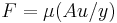 , where is the proportionality factor called the dynamic viscosity (also called absolute viscosity, or simply viscosity). The equation can be expressed in terms of shear stress;
 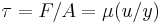 . The rate of shear deformation is
  and can be also written as a shear velocity, du/dy. Hence, through this method, the relation between the shear stress and the velocity gradient can be obtained.
James Clerk Maxwell called viscosity fugitive elasticity because of the analogy that elastic deformation opposes shear stress in solids, while in viscous fluids, shear stress is opposed by rate of deformation.
Viscosity measurement
Dynamic viscosity is measured with various types of rheometer. Close temperature control of the fluid is essential to accurate measurements, particularly in materials like lubricants, whose viscosity can double with a change of only 5 °C. For some fluids, it is a constant over a wide range of shear rates. These are Newtonian fluids.
The fluids without a constant viscosity are called Non-Newtonian fluids. Their viscosity cannot be described by a single number. Non-Newtonian fluids exhibit a variety of different correlations between shear stress and shear rate.
One of the most common instruments for measuring kinematic viscosity is the glass capillary viscometer.
In paint industries, viscosity is commonly measured with a Zahn cup, in which the efflux time is determined and given to customers. The efflux time can also be converted to kinematic viscosities (cSt) through the conversion equations.
Also used in paint, a Stormer viscometer uses load-based rotation in order to determine viscosity. The viscosity is reported in Krebs units (KU), which are unique to Stormer viscometers.
Vibrating viscometers can also be used to measure viscosity. These models such as the Dynatrol use vibration rather than rotation to measure viscosity.
Extensional viscosity can be measured with various rheometers that apply extensional stress
Volume viscosity can be measured with acoustic rheometer.
Units of measure
Dynamic viscosity
The usual symbol for dynamic viscosity used by mechanical engineers and fluid dynamicists is the Greek letter mu ()[8][9][10][11]. The symbol  is also used by chemists and IUPAC[12]. The SI physical unit of dynamic viscosity is the pascal-second (Pa·s), which is identical to kg·m−1·s−1. If a fluid with a viscosity of one Pa·s is placed between two plates, and one plate is pushed sideways with a shear stress of one pascal, it moves a distance equal to the thickness of the layer between the plates in one second.
The cgs physical unit for dynamic viscosity is the poise[13] (P), named after Jean Louis Marie Poiseuille. It is more commonly expressed, particularly in ASTM standards, as centipoise (cP). Water at 20 °C has a viscosity of 1.0020 cP.
- 1 P = 1 g·cm−1·s−1
The relation between poise and pascal-seconds is:
- 10 P = 1 kg·m−1·s−1 = 1 Pa·s
- 1 cP = 0.001 Pa·s = 1 mPa·s
The name 'poiseuille' (Pl) was proposed for this unit (after Jean Louis Marie Poiseuille who formulated Poiseuille's law of viscous flow), but not accepted internationally. Care must be taken in not confusing the poiseuille with the poise named after the same person.
Kinematic viscosity
In many situations, we are concerned with the ratio of the viscous force to the inertial force, the latter characterised by the fluid density ρ. This ratio is characterised by the kinematic viscosity (Greek letter nu,  ), defined as follows:
 ,
,
where is the dynamic viscosity (Pa·s) and  is the density (kg/m3), and is the kinematic viscosity (m2/s).
The cgs physical unit for kinematic viscosity is the stokes (St), named after George Gabriel Stokes. It is sometimes expressed in terms of centistokes (cSt or ctsk). In U.S. usage, stoke is sometimes used as the singular form.
- 1 stokes = 100 centistokes = 1 cm2·s−1 = 0.0001 m2·s−1.
- 1 centistokes = 1 mm2·s-1 = 10-6m2·s−1
The kinematic viscosity is sometimes referred to as diffusivity of momentum, because it is comparable to and has the same unit (m2s−1) as diffusivity of heat and diffusivity of mass. It is therefore used in dimensionless numbers which compare the ratio of the diffusivities.
Saybolt Universal Viscosity
At one time the petroleum industry relied on measuring kinematic viscosity by means of the Saybolt viscometer, and expressing kinematic viscosity in units of Saybolt Universal Seconds (SUS). [14] Kinematic viscosity in centistoke can be converted from SUS according to the arithmetic and the reference tabel provided in ASTM D 2161. It can also be converted in computerized method, or vice versa.[15]
Relation to Mean Free Path of Diffusing Particles
In relation to diffusion, the kinematic viscosity provides a better understanding of the behavior of mass transport of a dilute species. Viscosity is related to shear stress and the rate of shear in a fluid, which illustrates its dependence on the mean free path,  , of the diffusing particles.
From fluid mechanics, shear stress,  , is the rate of change of velocity with distance perpendicular to the direction of movement.
 .
.
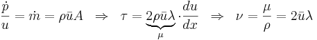
Interpreting shear stress as the time rate of change of momentum,p, per unit area (rate of momentum flux) of an arbitrary control surface gives
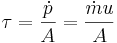 .
.
Further manipulation will show
where
 is the rate of change of mass
- is the density of the fluid
 is the average molecular speed
- is the dynamic viscosity.
Dynamic versus kinematic viscosity
Conversion between kinematic and dynamic viscosity is given by  .
.
For example,
- if
 0.0001 m2·s-1 and
  1000 kg m-3 then
  0.1 kg·m−1·s−1 = 0.1 Pa·s
 - if 1 St (= 1 cm2·s−1) and 1 g cm-3 then 1 g·cm−1·s−1 = 1 P
Example: viscosity of water
Because of its density of = 1 g/cm3 (varies slightly with temperature), and its dynamic viscosity is near 1 mPa·s (see #Viscosity of water section), the viscosity values of water are, to rough precision, all powers of ten:
Dynamic viscosity:
 = 1 mPa·s = 10-3 Pa·s = 1 cP = 10-2 poise
Kinematic viscosity:
 = 1 cSt = 10-2 stokes = 1 mm²/s
Molecular origins

The viscosity of a system is determined by how molecules constituting the system interact. There are no simple but correct expressions for the viscosity of a fluid. The simplest exact expressions are the Green-Kubo relations for the linear shear viscosity or the Transient Time Correlation Function expressions derived by Evans and Morriss in 1985. Although these expressions are each exact in order to calculate the viscosity of a dense fluid, using these relations requires the use of molecular dynamics computer simulations.
Gases
Viscosity in gases arises principally from the molecular diffusion that transports momentum between layers of flow. The kinetic theory of gases allows accurate prediction of the behavior of gaseous viscosity.
Within the regime where the theory is applicable:
- Viscosity is independent of pressure and
- Viscosity increases as temperature increases.
James Clerk Maxwell published a famous paper in 1866 using the kinetic theory of gases to study gaseous viscosity.[16]
Effect of temperature on the viscosity of a gas
Sutherland's formula can be used to derive the dynamic viscosity of an ideal gas as a function of the temperature:
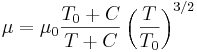
where:
- = dynamic viscosity in (Pa·s) at input temperature

 = reference viscosity in (Pa·s) at reference temperature
- = input temperature in kelvin
- = reference temperature in kelvin
 = Sutherland's constant for the gaseous material in question
Valid for temperatures between 0 < < 555 K with an error due to pressure less than 10% below 3.45 MPa
Sutherland's constant and reference temperature for some gases
| Gas |
[K] |
[K] |
[10-6 Pa s] |
|---|---|---|---|
| air | 120 | 291.15 | 18.27 |
| nitrogen | 111 | 300.55 | 17.81 |
| oxygen | 127 | 292.25 | 20.18 |
| carbon dioxide | 240 | 293.15 | 14.8 |
| carbon monoxide | 118 | 288.15 | 17.2 |
| hydrogen | 72 | 293.85 | 8.76 |
| ammonia | 370 | 293.15 | 9.82 |
| sulfur dioxide | 416 | 293.65 | 12.54 |
| helium | 79.4 [17] | 273 | 19 [18] |
(also see: [19])
Viscosity of a dilute gas
The Chapman-Enskog equation[20] may be used to estimate viscosity for a dilute gas. This equation is based on semi-theorethical assumption by Chapman and Enskoq. The equation requires three empirically determined parameters: the collision diameter (σ), the maximum energy of attraction divided by the Boltzmann constant (є/к) and the collision integral (ω(T*)).
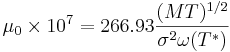
- T*=κT/ε Reduced temperature (dimensionless)
- = viscosity for dilute gas (uP)
 = molecular mass (g/mol)
- = temperature (K)
 = the collision diameter (Å)
 = the maximum energy of attraction divided by the Boltzmann constant (K)
 = the collision integral
Liquids
In liquids, the additional forces between molecules become important. This leads to an additional contribution to the shear stress though the exact mechanics of this are still controversial. Thus, in liquids:
- Viscosity is independent of pressure (except at very high pressure); and
- Viscosity tends to fall as temperature increases (for example, water viscosity goes from 1.79 cP to 0.28 cP in the temperature range from 0 °C to 100 °C); see temperature dependence of liquid viscosity for more details.
The dynamic viscosities of liquids are typically several orders of magnitude higher than dynamic viscosities of gases.
Viscosity of blends of liquids
The viscosity of the blend of two or more liquids can be estimated using the Refutas equation[21][22]. The calculation is carried out in three steps.
The first step is to calculate the Viscosity Blending Number (VBN) (also called the Viscosity Blending Index) of each component of the blend:
- (1)
![\mbox{VBN} = 14.534 \times ln[ln(v + 0.8)] + 10.975\,](/2009-wikipedia_en_wp1-0.7_2009-05/I/13b94da2c908803b06788fc44a57d36c.png)
where v is the kinematic viscosity in centistokes (cSt). It is important that the kinematic viscosity of each component of the blend be obtained at the same temperature.
The next step is to calculate the VBN of the blend, using this equation:
- (2)
![\mbox{VBN}_\mbox{Blend} = [x_A \times \mbox{VBN}_A] + [x_B \times \mbox{VBN}_B] + ... + [x_N \times \mbox{VBN}_N]\,](/2009-wikipedia_en_wp1-0.7_2009-05/I/127755015f8dae0457442415bd300781.png)
where  is the mass fraction of each component of the blend.
Once the viscosity blending number of a blend has been calculated using equation (2), the final step is to determine the kinematic viscosity of the blend by solving equation (1) for v:
- (3)
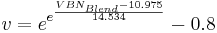
where  is the viscosity blending number of the blend.
Viscosity of selected substances
The viscosity of air and water are by far the two most important materials for aviation aerodynamics and shipping fluid dynamics. Temperature plays the main role in determining viscosity.
Viscosity of air
The viscosity of air depends mostly on the temperature. At 15.0 °C, the viscosity of air is 1.78 × 10⁻⁵ kg/(m·s) or 1.78 × 10⁻⁴ P. One can get the viscosity of air as a function of temperature from the Gas Viscosity Calculator
Viscosity of water
The viscosity of water is 8.90 × 10⁻⁴ Pa·s or 8.90 × 10⁻³ dyn·s/cm2 or 0.890 cP at about 25 °C.
As a function of temperature T (K): μ(Pa·s) = A × 10B/(T−C)
where A=2.414 × 10⁻⁵ Pa·s ; B = 247.8 K ; and C = 140 K.
Viscosity of water at different temperatures is listed below.
| Temperature
[°C] |
viscosity
[Pa·s] |
|---|---|
| 10 | 1.308 × 10⁻³ |
| 20 | 1.003 × 10⁻³ |
| 30 | 7.978 × 10⁻⁴ |
| 40 | 6.531 × 10⁻⁴ |
| 50 | 5.471 × 10⁻⁴ |
| 60 | 4.668 × 10⁻⁴ |
| 70 | 4.044 × 10⁻⁴ |
| 80 | 3.550 × 10⁻⁴ |
| 90 | 3.150 × 10⁻⁴ |
| 100 | 2.822 × 10⁻⁴ |
Viscosity of various materials


Some dynamic viscosities of Newtonian fluids are listed below:
| viscosity
[Pa·s] |
|
|---|---|
| hydrogen | 8.4 × 10⁻⁶ |
| air | 17.4 × 10⁻⁶ |
| xenon | 2.12 × 10⁻⁵ |
| viscosity
[Pa·s] |
viscosity
[cP] |
|
|---|---|---|
| acetone* | 3.06 × 10⁻⁴ | 0.306 |
| benzene* | 6.04 × 10⁻⁴ | 0.604 |
| blood | 3 to 4 × 10⁻³[23] | 1,37[24] |
| castor oil* | 0.985 | 985 |
| corn syrup* | 1.3806 | 1380.6 |
| ethanol* | 1.074 × 10⁻³ | 1.074 |
| ethylene glycol | 1.61 × 10⁻² | 16.1 |
| glycerol | 1.5 | 1500 |
| HFO-380 | 2.022 | 2022 |
| mercury* | 1.526 × 10⁻³ | 1.526 |
| methanol* | 5.44 × 10⁻⁴ | 0.544 |
| nitrobenzene* | 1.863 × 10⁻³ | 1.863 |
| liquid nitrogen @ 77K | 1.58 × 10⁻⁴ | 0.158 |
| propanol* | 1.945 × 10⁻³ | 1.945 |
| olive oil | .081 | 81 |
| pitch | 2.3 × 10⁸ | 2.3 × 10¹¹ |
| sulfuric acid* | 2.42 × 10⁻² | 24.2 |
| water | 8.94 × 10⁻⁴ | 0.894 |
* Data from CRC Handbook of Chemistry and Physics, 73rd edition, 1992-1993.
Fluids with variable compositions, such as honey, can have a wide range of viscosities.
| viscosity
[cP] |
|
|---|---|
| honey | 2,000–10,000 |
| molasses | 5,000–10,000 |
| molten glass | 10,000–1,000,000 |
| chocolate syrup | 10,000–25,000 |
| molten chocolate* | 45,000–130,000 [25] |
| ketchup* | 50,000–100,000 |
| peanut butter | ~250,000 |
| shortening* | ~250,000 |
* These materials are highly non-Newtonian.
Viscosity of solids
On the basis that all solids such as granite[26] flow to a small extent in response to shear stress, some researchers[27] have contended that substances known as amorphous solids, such as glass and many polymers, may be considered to have viscosity. This has led some to the view that solids are simply liquids with a very high viscosity, typically greater than 1012 Pa·s. This position is often adopted by supporters of the widely held misconception that glass flow can be observed in old buildings. This distortion is more likely the result of the glass making process rather than the viscosity of glass.[28]
However, others argue that solids are, in general, elastic for small stresses while fluids are not.[29] Even if solids flow at higher stresses, they are characterized by their low-stress behavior. Viscosity may be an appropriate characteristic for solids in a plastic regime. The situation becomes somewhat confused as the term viscosity is sometimes used for solid materials, for example Maxwell materials, to describe the relationship between stress and the rate of change of strain, rather than rate of shear.
These distinctions may be largely resolved by considering the constitutive equations of the material in question, which take into account both its viscous and elastic behaviors. Materials for which both their viscosity and their elasticity are important in a particular range of deformation and deformation rate are called viscoelastic. In geology, earth materials that exhibit viscous deformation at least three times greater than their elastic deformation are sometimes called rheids.
Viscosity of amorphous materials

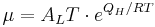
Viscous flow in amorphous materials (e.g. in glasses and melts)[31][32][33] is a thermally activated process:
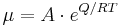
where  is activation energy, is temperature,
  is the molar gas constant and
  is approximately a constant.
The viscous flow in amorphous materials is characterized by a deviation from the Arrhenius-type behavior: changes from a high value  at low temperatures (in the glassy state) to a low value
  at high temperatures (in the liquid state). Depending on this change, amorphous materials are classified as either
- strong when:
 or
or - fragile when:
The fragility of amorphous materials is numerically characterized by the Doremus’ fragility ratio:
and strong material have  whereas fragile materials have
The viscosity of amorphous materials is quite exactly described by a two-exponential equation:
![\mu = A_1 \cdot T \cdot [1 + A_2 \cdot e^{B/RT}] \cdot [1 + C \cdot e^{D/RT}]](/2009-wikipedia_en_wp1-0.7_2009-05/I/37730dd19ce5d876dd529ca7a7c2e7da.png)
with constants  and
and  related to thermodynamic parameters of joining bonds of an amorphous material.
Not very far from the glass transition temperature,  , this equation can be approximated by a Vogel-Tammann-Fulcher (VTF) equation or a Kohlrausch-type stretched-exponential law.
If the temperature is significantly lower than the glass transition temperature,  , then the two-exponential equation simplifies to an Arrhenius type equation:
with:
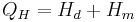
where  is the enthalpy of formation of broken bonds (termed configurons) and
  is the enthalpy of their motion. When the temperature is less than the glass transition temperature, , the activation energy of viscosity is high because the amorphous materials are in the glassy state and most of their joining bonds are intact.
If the temperature is highly above the glass transition temperature,  , the two-exponential equation also simplifies to an Arrhenius type equation:
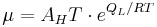
with:

When the temperature is higher than the glass transition temperature, , the activation energy of viscosity is low because amorphous materials are melt and have most of their joining bonds broken which facilitates flow.
Volume (bulk) viscosity
The negative-one-third of the trace of the stress tensor is often identified with the thermodynamic pressure,
,
which only depends upon the equilibrium state potentials like temperature and density (equation of state). In general, the trace of the stress tensor is the sum of thermodynamic pressure contribution plus another contribution which is proportional to the divergence of the velocity field. This constant of proportionality is called the volume viscosity.
Eddy viscosity
In the study of turbulence in fluids, a common practical strategy for calculation is to ignore the small-scale vortices (or eddies) in the motion and to calculate a large-scale motion with an eddy viscosity that characterizes the transport and dissipation of energy in the smaller-scale flow (see large eddy simulation). Values of eddy viscosity used in modeling ocean circulation may be from 5x10⁴ to 106 Pa·s depending upon the resolution of the numerical grid.
Fluidity
The reciprocal of viscosity is fluidity, usually symbolized by  or
or  , depending on the convention used, measured in reciprocal poise (cm·s·g-1), sometimes called the rhe. Fluidity is seldom used in engineering practice.
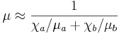
The concept of fluidity can be used to determine the viscosity of an ideal solution. For two components  and
and  , the fluidity when and are mixed is
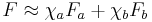
which is only slightly simpler than the equivalent equation in terms of viscosity:
where  and
and  is the mole fraction of component and respectively, and
  and
and  are the components pure viscosities.
The linear viscous stress tensor
(See Hooke's law and strain tensor for an analogous development for linearly elastic materials.)
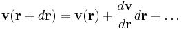
Viscous forces in a fluid are a function of the rate at which the fluid velocity is changing over distance. The velocity at any point  is specified by the velocity field
  . The velocity at a small distance
  from point may be written as a Taylor series:
where  is shorthand for the dyadic product of the del operator and the velocity:
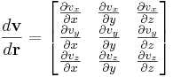
This is just the Jacobian of the velocity field. Viscous forces are the result of relative motion between elements of the fluid, and so are expressible as a function of the velocity field. In other words, the forces at are a function of and all derivatives of at that point. In the case of linear viscosity, the viscous force will be a function of the Jacobian tensor alone. For almost all practical situations, the linear approximation is sufficient.
If we represent x, y, and z by indices 1, 2, and 3 respectively, the i,j component of the Jacobian may be written as  where
where  is shorthand for
  . Note that when the first and higher derivative terms are zero, the velocity of all fluid elements is parallel, and there are no viscous forces.
Any matrix may be written as the sum of an antisymmetric matrix and a symmetric matrix, and this decomposition is independent of coordinate system, and so has physical significance. The velocity field may be approximated as:

where Einstein notation is now being used in which repeated indices in a product are implicitly summed. The second term from the right is the asymmetric part of the first derivative term, and it represents a rigid rotation of the fluid about with angular velocity  where:
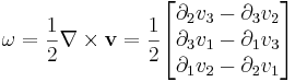
For such a rigid rotation, there is no change in the relative positions of the fluid elements, and so there is no viscous force associated with this term. The remaining symmetric term is responsible for the viscous forces in the fluid. Assuming the fluid is isotropic (i.e. its properties are the same in all directions), then the most general way that the symmetric term (the rate-of-strain tensor) can be broken down in a coordinate-independent (and therefore physically real) way is as the sum of a constant tensor (the rate-of-expansion tensor) and a traceless symmetric tensor (the rate-of-shear tensor):
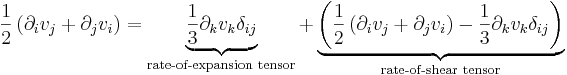
where  is the unit tensor. The most general linear relationship between the stress tensor
  and the rate-of-strain tensor is then a linear combination of these two tensors:[34]
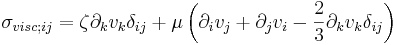
where  is the coefficient of bulk viscosity (or "second viscosity") and is the coefficient of (shear) viscosity.
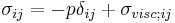
The forces in the fluid are due to the velocities of the individual molecules. The velocity of a molecule may be thought of as the sum of the fluid velocity and the thermal velocity. The viscous stress tensor described above gives the force due to the fluid velocity only. The force on an area element in the fluid due to the thermal velocities of the molecules is just the hydrostatic pressure. This pressure term ( ) must be added to the viscous stress tensor to obtain the total stress tensor for the fluid.
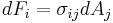
The infinitesimal force  on an infinitesimal area
  is then given by the usual relationship:
See also
- Deborah number
- Dilatant
- Hyperviscosity syndrome
- Inviscid flow
- Reynold's number
- Rheology
- Thixotropy
- Viscometer
- Viscometry
- Viscoelasticity
- Viscosity index
- Joback method (Estimation of the liquid viscosity from molecular structure)
References
- ↑ Symon, Keith (1971). Mechanics (Third Edition ed.). Addison-Wesley. ISBN 0-201-07392-7.
- ↑ The Online Etymology Dictionary
- ↑ Happel, J. and Brenner , H. "Low Reynolds number hydrodynamics", Prentice-Hall, (1965)
- ↑ Landau, L.D. and Lifshitz, E.M. "Fluid mechanics", Pergamon Press,(1959)
- ↑ Barnes, H.A. "A Handbook of Elementary Rheology", Institute of Non-Newtonian Fluid mechanics, UK (2000)
- ↑ Raymond A. Serway (1996). Physics for Scientists & Engineers (4th Edition ed.). Saunders College Publishing. ISBN 0-03-005932-1.
- ↑ Dukhin, A.S. and Goetz, P.J. "Ultrasound for characterizing colloids", Elsevier, (2002)
- ↑ ASHRAE handbook, 1989 edition
- ↑ Streeter & Wylie Fluid Mechanics, McGraw-Hill, 1981
- ↑ Holman Heat Transfer, McGraw-Hill, 2002
- ↑ Incropera & DeWitt, Fundamentals of Heat and Mass Transfer, Wiley, 1996
- ↑ IUPAC Gold Book, Definition of (dynamic) viscosity
- ↑ IUPAC definition of the Poise
- ↑ ASTM D 2161, Page one,(2005)
- ↑ Quantities and Units of Viscosity
- ↑ Maxwell, J. C. (1866), "On the viscosity or internal friction of air and other gases", Philosophical Transactions of the Royal Society of London 156: 249–268, doi:
- ↑ data constants for sutherland's formula
- ↑ Viscosity of liquids and gases
- ↑ http://www.epa.gov/EPA-AIR/2005/July/Day-13/a11534d.htm
- ↑ J.O. Hirshfelder, C.F. Curtis and R.B. Bird (1964). Molecular theory of gases and liquids (First Edition ed.). Wiley. ISBN 0-471-40065-3.
- ↑ Robert E. Maples (2000). Petroleum Refinery Process Economics (2nd Edition ed.). Pennwell Books. ISBN 0-87814-779-9.
- ↑ C.T. Baird (1989), Guide to Petroleum Product Blending, HPI Consultants, Inc. HPI website
- ↑ [www.geocities.com/placenta_rb/1-1.html geocities.com - Study and Validation of a Model of Fetoplacental Circulation - Rheology of fetal blood]
- ↑ Viscosity. The Physics Hypertextbook. by Glenn Elert
- ↑ "Chocolate Processing". Brookfield Engineering website. Retrieved on 2007-12-03.
- ↑ Kumagai, Naoichi; Sadao Sasajima, Hidebumi Ito (15 February 1978). "Long-term Creep of Rocks: Results with Large Specimens Obtained in about 20 Years and Those with Small Specimens in about 3 Years". Journal of the Society of Materials Science (Japan) (Japan Energy Society) 27 (293): 157–161. http://translate.google.com/translate?hl=en&sl=ja&u=http://ci.nii.ac.jp/naid/110002299397/&sa=X&oi=translate&resnum=4&ct=result&prev=/search%3Fq%3DIto%2BHidebumi%26hl%3Den. Retrieved on 2008-06-16.
- ↑ Elert, Glenn. "Viscosity". The Physics Hypertextbook.
- ↑ "Antique windowpanes and the flow of supercooled liquids", by Robert C. Plumb, (Worcester Polytech. Inst., Worcester, MA, 01609, USA), J. Chem. Educ. (1989), 66 (12), 994-6
- ↑ Gibbs, Philip. "Is Glass a Liquid or a Solid?". Retrieved on 2007-07-31.
- ↑ Viscosity calculation of glasses
- ↑ R.H.Doremus (2002). "Viscosity of silica". J. Appl. Phys. 92 (12): 7619–7629. doi:. ISSN 0021-8979.
- ↑ M.I. Ojovan and W.E. Lee (2004). "Viscosity of network liquids within Doremus approach". J. Appl. Phys. 95 (7): 3803–3810. doi:. ISSN 0021-8979.
- ↑ M.I. Ojovan, K.P. Travis and R.J. Hand (2000). "Thermodynamic parameters of bonds in glassy materials from viscosity-temperature relationships". J. Phys.: Condensed matter 19 (41): 415107. doi:. ISSN 0953-8984.
- ↑ L.D. Landau and E.M. Lifshitz (translated from Russian by J.B. Sykes and W.H. Reid) (1997). Fluid Mechanics (2nd Edition ed.). Butterworth Heinemann. ISBN 0-7506-2767-0.
Additional reading
- Massey, B. S. (1983). Mechanics of Fluids (Fifth Edition ed.). Van Nostrand Reinhold (UK). ISBN 0-442-30552-4.
External links
- Fluid Characteristics Chart A table of viscosities and vapor pressures for various fluids
- Gas Dynamics Toolbox Calculate coefficient of viscosity for mixtures of gases
- Glass Viscosity Measurement Viscosity measurement, viscosity units and fixpoints, glass viscosity calculation
- Kinematic Viscosity conversion between kinematic and dynamic viscosity.
- Physical Characteristics of Water A table of water viscosity as a function of temperature
- Vogel-Tammann-Fulcher Equation Parameters
|
|||||