Propositional calculus
- This is a technical mathematical article about the area of mathematical logic variously known as "propositional calculus" or "propositional logic".
In logic and mathematics, a propositional calculus (or a sentential calculus) is a formal system in which formulae representing propositions can be formed by combining atomic propositions using logical connectives, and a system of formal proof rules allows certain formulæ to be established as "theorems".
In logic and philosophy, propositional calculus is often intended to symbolize rational deduction.
Terminology
In general terms, a calculus is a formal system that consists of a set of syntactic expressions (well-formed formulæ or wffs), a distinguished subset of these expressions (axioms), plus a set of formal rules that define a specific binary relation, intended to be interpreted as logical equivalence, on the space of expressions.
When the formal system is intended to be a logical system, the expressions are meant to be interpreted as statements, and the rules, known as inference rules, are typically intended to be truth-preserving. In this setting, the rules (which may include axioms) can then be used to derive ("infer") formulæ representing true statements from given formulæ representing true statements.
The set of axioms may be empty, a nonempty finite set, a countably infinite set, or be given by axiom schemata. A formal grammar recursively defines the expressions and well-formed formulæ (wffs) of the language. In addition a semantics may be given which defines truth and valuations (or interpretations).
The language of a propositional calculus consists of (1) a set of primitive symbols, variously referred to as atomic formulae, placeholders, proposition letters, or variables, and (2) a set of operator symbols, variously interpreted as logical operators or logical connectives. A well-formed formula (wff) is any atomic formula or any formula that can be built up from atomic formulæ by means of operator symbols according to the rules of the grammar.
Outline
The following outlines a standard propositional calculus. Many different formulations exist which are all more or less equivalent but differ in the details of (1) their language, that is, the particular collection of primitive symbols and operator symbols, (2) the set of axioms, or distinguished formulæ, and (3) the set of inference rules.
Generic description of a propositional calculus
A propositional calculus is a formal system 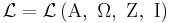 , whose formulæ are constructed in the following manner:
- The alpha set
 is a finite set of elements called proposition symbols or propositional variables. Syntactically speaking, these are the most basic elements of the formal language
  , otherwise referred to as atomic formulæ or terminal elements. In the examples to follow, the elements of are typically the letters
  ,
,  ,
,  , and so on.
- The omega set
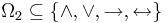
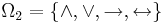
 is a finite set of elements called operator symbols or logical connectives. The set is partitioned into disjoint subsets as follows:
-
-
 .
.
-
- In this partition,
 is the set of operator symbols of arity
  .
.
- In the more familiar propositional calculi, is typically partitioned as follows:
-
-
 ,
,
-
-
-
 .
.
-
- A frequently adopted option treats the constant logical values as operators of arity zero, thus:
-
-
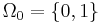 .
.
-
- Some writers use the tilde (~) instead of (
 ); and some use the ampersand (&) or
  instead of
  . Notation varies even more for the set of logical values, with symbols like {false, true}, {F, T}, or
  all being seen in various contexts instead of {0, 1}.
- Depending on the precise formal grammar or the grammar formalism that is being used, syntactic auxiliaries like the left parenthesis, "(", and the right parentheses, ")", may be necessary to complete the construction of formulæ.
- The language of , also known as its set of formulæ, well-formed formulas or wffs, is inductively or recursively defined by the following rules:
-
- Base. Any element of the alpha set is a formula of .
- Step (a). If is a formula, then
 is a formula.
 - Step (b). If and are formulæ, then
 ,
,  ,
,  , and
, and  are formulæ.
 - Close. Nothing else is a formula of .
- Base. Any element of the alpha set
- Repeated applications of these rules permits the construction of complex formulæ. For example:
-
- By rule 1, is a formula.
- By rule 2, is a formula.
- By rule 1, is a formula.
- By rule 3,
 is a formula.
- By rule 1,
- The zeta set
 is a finite set of transformation rules that are called inference rules when they acquire logical applications.
- The iota set
 is a finite set of initial points that are called axioms when they receive logical interpretations.
Example 1. Simple axiom system
Let 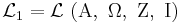 , where
  are defined as follows:
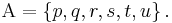
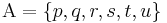
- The alpha set
 , is a finite set of symbols that is large enough to supply the needs of a given discussion, for example:
- Of the three connectives for conjunction, disjunction, and implication (,
 , and
, and  ), one can be taken as primitive and the other two can be defined in terms of it and negation (). Indeed, all of the logical connectives can be defined in terms of a sole sufficient operator. The biconditional (
 ) can of course be defined in terms of conjunction and implication, with
  defined as
  .
.
Adopting negation and implication as the two primitive operations of a propositional calculus is tantamount to having the omega set partition as follows:


- An axiom system discovered by Jan Łukasiewicz formulates a propositional calculus in this language as follows. The axioms are all substitution instances of:

- The rule of inference is modus ponens (i.e. from and
 , infer ). Then
  is defined as
  , and
, and  is defined as
  .
.
Example 2. Natural deduction system
Let 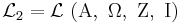 , where are defined as follows:
- The alpha set , is a finite set of symbols that is large enough to supply the needs of a given discussion, for example:
- The omega set partitions as follows:
In the following example of a propositional calculus, the transformation rules are intended to be interpreted as the inference rules of a so-called natural deduction system. The particular system presented here has no initial points, which means that its interpretation for logical applications derives its theorems from an empty axiom set.
- The set of initial points is empty, that is,

- The set of transformation rules, , is described as follows:
Our propositional calculus has ten inference rules. These rules allow us to derive other true formulae given a set of formulae that are assumed to be true. The first nine simply state that we can infer certain wffs from other wffs. The last rule however uses hypothetical reasoning in the sense that in the premise of the rule we temporarily assume an (unproven) hypothesis to be part of the set of inferred formulae to see if we can infer a certain other formula. Since the first nine rules don't do this they are usually described as non-hypothetical rules, and the last one as a hypothetical rule.
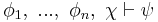
- Reductio ad absurdum (negation introduction)
- From , if accepting (q) leads to a proof that
 , infer
  .
. - Double negative elimination
- From
 , infer .
 - Conjunction introduction
- From and , infer
 .
. - From and , infer
 .
. - Conjunction elimination
- From , infer
- From , infer .
- Disjunction introduction
- From , infer

- From , infer
 .
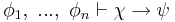
. - Disjunction elimination
- From ,
 ,
,  , infer .
 - Biconditional introduction
- From ,
 , infer
  .
. - Biconditional elimination
- From , infer
 ;
; - From , infer .
- Modus ponens (conditional elimination)
- From , , infer .
- Conditional proof (conditional introduction)
- If accepting allows a proof of , infer .
| Basic and Derived Argument Forms | ||
|---|---|---|
| Name | Sequent | Description |
| Modus Ponens | 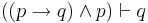 |
If p then q; p; therefore q |
| Modus Tollens | 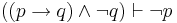 |
If p then q; not q; therefore not p |
| Hypothetical Syllogism |  |
If p then q; if q then r; therefore, if p then r |
| Disjunctive Syllogism | 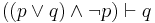 |
Either p or q, or both; not p; therefore, q |
| Constructive Dilemma |  |
If p then q; and if r then s; but p or r; therefore q or s |
| Destructive Dilemma |  |
If p then q; and if r then s; but not q or not s; therefore not p or not r |
| Bidirectional Dilemma |  |
If p then q; and if r then s; but p or not s; therefore q or not r |
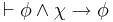
| Simplification |  |
p and q are true; therefore p is true |
| Conjunction | 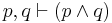 |
p and q are true separately; therefore they are true conjointly |
| Addition |  |
p is true; therefore the disjunction (p or q) is true |
| Composition |  |
If p then q; and if p then r; therefore if p is true then q and r are true |
| De Morgan's Theorem (1) | 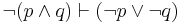 |
The negation of (p and q) is equiv. to (not p or not q) |
| De Morgan's Theorem (2) | 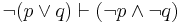 |
The negation of (p or q) is equiv. to (not p and not q) |
| Commutation (1) | 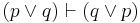 |
(p or q) is equiv. to (q or p) |
| Commutation (2) | 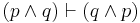 |
(p and q) is equiv. to (q and p) |
| Commutation (3) |  |
(p is equiv. to q) is equiv. to (q is equiv. to p) |
| Association (1) |  |
p or (q or r) is equiv. to (p or q) or r |
| Association (2) |  |
p and (q and r) is equiv. to (p and q) and r |
| Distribution (1) |  |
p and (q or r) is equiv. to (p and q) or (p and r) |
| Distribution (2) |  |
p or (q and r) is equiv. to (p or q) and (p or r) |
| Double Negation |  |
p is equivalent to the negation of not p |
| Transposition |  |
If p then q is equiv. to if not q then not p |
| Material Implication |  |
If p then q is equiv. to not p or q |
| Material Equivalence (1) |  |
(p is equiv. to q) means (if p is true then q is true) and (if q is true then p is true) |
| Material Equivalence (2) |  |
(p is equiv. to q) means either (p and q are true) or (both p and q are false) |
| Material Equivalence (3) |  |
(p is equiv. to q) means, both (p or not q is true) and (not p or q is true) |
| Exportation |  |
from (if p and q are true then r is true) we can prove (if q is true then r is true, if p is true) |
| Importation |  |
|
| Tautology (1) |  |
p is true is equiv. to p is true or p is true |
| Tautology (2) |  |
p is true is equiv. to p is true and p is true |
| Tertium non datur (Law of Excluded Middle) |  |
p or not p is true |
| Law of Non-Contradiction |  |
p and not p is false, is a true statement |
Proofs in propositional calculus
One of the main uses of a propositional calculus, when interpreted for logical applications, is to determine relations of logical equivalence between propositional formulæ. These relationships are determined by means of the available transformation rules, sequences of which are called derivations or proofs.
In the discussion to follow, a proof is presented as a sequence of numbered lines, with each line consisting of a single formula followed by a reason or justification for introducing that formula. Each premise of the argument, that is, an assumption introduced as an hypothesis of the argument, is listed at the beginning of the sequence and is marked as a "premise" in lieu of other justification. The conclusion is listed on the last line. A proof is complete if every line follows from the previous ones by the correct application of a transformation rule. (For a contrasting approach, see proof-trees).
Example of a proof
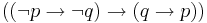
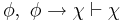
- To be shown that
 .
.
- One possible proof of this (which, though valid, happens to contain more steps than are necessary) may be arranged as follows:
| Example of a Proof | ||
|---|---|---|
| Number | Formula | Reason |
| 1 |  |
premise |
| 2 |  |
From (1) by disjunction introduction |
| 3 |  |
From (1) and (2) by conjunction introduction |
| 4 | |
From (3) by conjunction elimination |
| 5 |  |
Summary of (1) through (4) |
| 6 |  |
From (5) by conditional proof |
Interpret as "Assuming , infer ". Read as "Assuming nothing, infer that implies ", or "It is a tautology that implies ", or "It is always true that implies ".
Soundness and completeness of the rules
The crucial properties of this set of rules are that they are sound and complete. Informally this means that the rules are correct and that no other rules are required. These claims can be made more formal as follows.
We define a truth assignment as a function that maps propositional variables to true or false. Informally such a truth assignment can be understood as the description of a possible state of affairs (or possible world) where certain statements are true and others are not. The semantics of formulae can then be formalized by defining for which "state of affairs" they are considered to be true, which is what is done by the following definition.
We define when such a truth assignment satisfies a certain wff with the following rules:
- satisfies the propositional variable
 if and only if
- satisfies
 if and only if does not satisfy
- satisfies
 if and only if satisfies both and
- satisfies
 if and only if satisfies at least one of either or
 - satisfies
 if and only if it is not the case that satisfies but not
 - satisfies
 if and only if satisfies both and or satisfies neither one of them
With this definition we can now formalize what it means for a formula  to be implied by a certain set
  of formulae. Informally this is true if in all worlds that are possible given the set of formulae the formula also holds. This leads to the following formal definition: We say that a set of wffs semantically entails (or implies) a certain wff if all truth assignments that satisfy all the formulae in also satisfy .
Finally we define syntactical entailment such that  is syntactically entailed by if and only if we can derive it with the inference rules that were presented above in a finite number of steps. This allows us to formulate exactly what it means for the set of inference rules to be sound and complete:
- Soundness
- If the set of wffs syntactically entails wff then semantically entails
- Completeness
- If the set of wffs semantically entails wff then syntactically entails
For the above set of rules this is indeed the case.
Sketch of a soundness proof
(For most logical systems, this is the comparatively "simple" direction of proof)
Notational conventions: Let "G" be a variable ranging over sets of sentences. Let "A", "B", and "C" range over sentences. For "G syntactically entails A" we write "G proves A". For "G semantically entails A" we write "G implies A".
We want to show: (A)(G)(if G proves A, then G implies A).
We note that "G proves A" has an inductive definition, and that gives us the immediate resources for demonstrating claims of the form "If G proves A, then ...". So our proof proceeds by induction.
- I. Basis. Show: If A is a member of G, then G implies A.
- II. Basis. Show: If A is an axiom, then G implies A.
- III. Inductive step (induction on n, the length of the proof):
-
- (a) Assume for arbitrary G and A that if G proves A in n or fewer steps, then G implies A.
- (b) For each possible application of a rule of inference at step n+1, leading to a new theorem B, show that G implies B.
Notice that Basis Step II can be omitted for natural deduction systems because they have no axioms. When used, Step II involves showing that each of the axioms is a (semantic) logical truth.
The Basis step(s) demonstrate(s) that the simplest provable sentences from G are also implied by G, for any G. (The is simple, since the semantic fact that a set implies any of its members, is also trivial.) The Inductive step will systematically cover all the further sentences that might be provable—by considering each case where we might reach a logical conclusion using an inference rule—and shows that if a new sentence is provable, it is also logically implied. (For example, we might have a rule telling us that from "A" we can derive "A or B". In III.(a) We assume that if A is provable it is implied. We also know that if A is provable then "A or B" is provable. We have to show that then "A or B" too is implied. We do so by appeal to the semantic definition and the assumption we just made. A is provable from G, we assume. So it is also implied by G. So any semantic valuation making all of G true makes A true. But any valuation making A true makes "A or B" true, by the defined semantics for "or". So any valuation which makes all of G true makes "A or B" true. So "A or B" is implied.) Generally, the Inductive step will consist of a lengthy but simple case-by-case analysis of all the rules of inference, showing that each "preserves" semantic implication.
By the definition of provability, there are no sentences provable other than by being a member of G, an axiom, or following by a rule; so if all of those are semantically implied, the deduction calculus is sound.
Sketch of completeness proof
(This is usually the much harder direction of proof.)
We adopt the same notational conventions as above.
We want to show: If G implies A, then G proves A. We proceed by contraposition: We show instead that If G does not prove A then G does not imply A.
- I. G does not prove A. (Assumption)
- II. If G does not prove A, then we can construct an (infinite) "Maximal Set", G*, which is a superset of G and which also does not prove A.
- (a)Place an "ordering" on all the sentences in the language. (e.g., alphabetical ordering), and number them E1, E2, ...
- (b)Define a series Gn of sets (G0, G1 ... ) inductively, as follows. (i)G0 = G. (ii) If {Gk, E(k+1)} proves A, then G(k+1) = Gk. (iii) If {Gk, E(k+1)} does not prove A, then G(k+1) = {Gk, E(k+1)}
- (c)Define G* as the union of all the Gn. (That is, G* is the set of all the sentences that are in any Gn).
- (d) It can be easily shown that (i) G* contains (is a superset of) G (by (b.i)); (ii) G* does not prove A (because if it proves A then some sentence was added to some Gn which caused it to prove A; but this was ruled out by definition); and (iii) G* is a "Maximal Set" (with respect to A): If any more sentences whatever were added to G*, it would prove A. (Because if it were possible to add any more sentences, they should have been added when they were encountered during the construction of the Gn, again by definition)
- III. If G* is a Maximal Set (wrt A), then it is "truth-like". This means that it contains the sentence "C" only if it does not contain the sentence not-C; If it contains "C" and contains "If C then B" then it also contains "B"; and so forth.
- IV. If G* is truth-like there is a "G*-Canonical" valuation of the language: one that makes every sentence in G* true and everything outside G* false while still obeying the laws of semantic composition in the language.
- V. A G*-canonical valuation will make our original set G all true, and make A false.
- VI. If there is a valuation on which G are true and A is false, then G does not (semantically) imply A.
QED
Another outline for a completeness proof
If a formula is a tautology, then there is a truth table for it which shows that each valuation yields the value true for the formula. Consider such a valuation. By mathematical induction on the length of the subformulae, show that the truth or falsity of the subformula follows from the truth or falsity (as appropriate for the valuation) of each propositional variable in the subformula. Then combine the lines of the truth table together two at a time by using "(P is true implies S) implies ((P is false implies S) implies S)". Keep repeating this until all dependencies on propositional variables have been eliminated. The result is that we have proved the given tautology. Since every tautology is provable, the logic is complete.
Alternative calculus
It is possible to define another version of propositional calculus, which defines most of the syntax of the logical operators by means of axioms, and which uses only one inference rule.
Axioms
Let ,  and
and  stand for well-formed formulæ. (The wffs themselves would not contain any Greek letters, but only capital Roman letters, connective operators, and parentheses.) Then the axioms are as follows:
| Axioms | ||
|---|---|---|
| Name | Axiom Schema | Description |
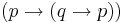
| THEN-1 |  |
Add hypothesis , implication introduction |
| THEN-2 |  |
Distribute hypothesis over implication |
| AND-1 |  |
Eliminate conjunction |
| AND-2 |  |
|
| AND-3 |  |
Introduce conjunction |
| OR-1 |  |
Introduce disjunction |
| OR-2 |  |
|
| OR-3 | ( |
Eliminate disjunction |
| NOT-1 | ( |
Introduce negation |
| NOT-2 | 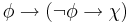 |
Eliminate negation |
| NOT-3 |  |
Excluded middle, classical logic |
| IFF-1 | (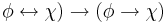 |
Eliminate equivalence |
| IFF-2 | ( |
|
| IFF-3 | ( |
Introduce equivalence |
Axiom THEN-2 may be considered to be a "distributive property of implication with respect to implication."
Axioms AND-1 and AND-2 correspond to "conjunction elimination". The relation between AND-1 and AND-2 reflects the commutativity of the conjunction operator.
Axiom AND-3 corresponds to "conjunction introduction."
Axioms OR-1 and OR-2 correspond to "disjunction introduction." The relation between OR-1 and OR-2 reflects the commutativity of the disjunction operator.
Axiom NOT-1 corresponds to "reductio ad absurdum."
Axiom NOT-2 says that "anything can be deduced from a contradiction."
Axiom NOT-3 is called "tertium non datur" (Latin: "a third is not given") and reflects the semantic valuation of propositional formulae: a formula can have a truth-value of either true or false. There is no third truth-value, at least not in classical logic. Intuitionistic logicians do not accept the axiom NOT-3.
Inference rule
The inference rule is modus ponens:
 .
.
Meta-inference rule
Let a demonstration be represented by a sequence, with hypotheses to the left of the turnstile and the conclusion to the right of the turnstile. Then the deduction theorem can be stated as follows:
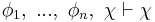
- If the sequence
- has been demonstrated, then it is also possible to demonstrate the sequence
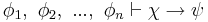 .
.
This deduction theorem (DT) is not itself formulated with propositional calculus: it is not a theorem of propositional calculus, but a theorem about propositional calculus. In this sense, it is a meta-theorem, comparable to theorems about the soundness or completeness of propositional calculus.
On the other hand, DT is so useful for simplifying the syntactical proof process that it can be considered and used as another inference rule, accompanying modus ponens. In this sense, DT corresponds to the natural conditional proof inference rule which is part of the first version of propositional calculus introduced in this article.
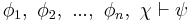
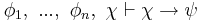
The converse of DT is also valid:
- If the sequence
- has been demonstrated, then it is also possible to demonstrate the sequence
in fact, the validity of the converse of DT is almost trivial compared to that of DT:
- If
- then
- 1:
- 2:
- 1:
- and from (1) and (2) can be deduced
- 3:
- 3:
- by means of modus ponens, Q.E.D.
The converse of DT has powerful implications: it can be used to convert an axiom into an inference rule. For example, the axiom AND-1,
can be transformed by means of the converse of the deduction theorem into the inference rule

which is conjunction elimination, one of the ten inference rules used in the first version (in this article) of the propositional calculus.
Example of a proof
The following is an example of a (syntactical) demonstration, involving only axioms THEN-1 and THEN-2:
Prove: A → A (Reflexivity of implication).
Proof:
- 1. (A → ((B → A) → A)) → ((A → (B → A)) → (A → A))
- Axiom THEN-2 with φ = A, χ = B → A, ψ = A
- 2. A → ((B → A) → A)
- Axiom THEN-1 with φ = A, χ = B → A
- 3. (A → (B → A)) → (A → A)
- From (1) and (2) by modus ponens.
- 4. A → (B → A)
- Axiom THEN-1 with φ = A, χ = B
- 5. A → A
- From (3) and (4) by modus ponens.
Equivalence to equational logics
The preceding alternative calculus is an example of a Hilbert-style deduction system. In the case of propositional systems the axioms are terms built with logical connectives and the only inference rule is modus ponens. Equational logic as standardly used informally in high school algebra is a different kind of calculus from Hilbert systems. Its theorems are equations and its inference rules express the properties of equality, namely that it is a congruence on terms that admits substitution.
Classical propositional calculus as described above is equivalent to Boolean algebra, while intuitionistic propositional calculus is equivalent to Heyting algebra. The equivalence is shown by translation in each direction of the theorems of the respective systems. Theorems Φ of classical or intuitionistic propositional calculus are translated as equations Φ = 1 of Boolean or Heyting algebra respectively. Conversely theorems  of Boolean or Heyting algebra are translated as theorems
 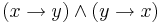 of classical or propositional calculus respectively, for which
  is a standard abbreviation. In the case of Boolean algebra can also be translated as
  , but this translation is incorrect intuitionistically.
In both Boolean and Heyting algebra, inequality  can be used in place of equality. The equality is expressible as a pair of inequalities and
  . Conversely the inequality is expressible as the equality
  , or as
  . The significance of inequality for Hilbert-style systems is that it corresponds to the latter's deduction or entailment symbol
  . An entailment
is translated in the inequality version of the algebraic framework as

Conversely the algebraic inequality is translated as the entailment
The difference between implication  and inequality or entailment or
  is that the former is internal to the logic while the latter is external. Internal implication between two terms is another term of the same kind. Entailment as external implication between two terms expresses a metatruth outside the language of the logic, and is considered part of the metalanguage. Even when the logic under study is intuitionistic, entailment is ordinarily understood classically as two-valued: either the left side entails, or is less-or-equal to, the right side, or it is not.
Similar but more complex translations to and from algebraic logics are possible for natural deduction systems as described above and for the sequent calculus. The entailments of the latter can be interpreted as two-valued, but a more insightful interpretation is as a set, the elements of which can be understood as abstract proofs organized as the morphisms of a category. In this interpretation the cut rule of the sequent calculus corresponds to composition in the category. Boolean and Heyting algebras enter this picture as special categories having at most one morphism per homset, i.e. one proof per entailment, corresponding to the idea that existence of proofs is all that matters: any proof will do and there is no point in distinguishing them.
Graphical calculi
It is possible to generalize the definition of a formal language from a set of finite sequences over a finite basis to include many other sets of mathematical structures, so long as they are built up by finitary means from finite materials. What's more, many of these families of formal structures are especially well-suited for use in logic.
For example, there are many families of graphs that are close enough analogues of formal languages that the concept of a calculus is quite easily and naturally extended to them. Indeed, many species of graphs arise as parse graphs in the syntactic analysis of the corresponding families of text structures. The exigencies of practical computation on formal languages frequently demand that text strings be converted into pointer structure renditions of parse graphs, simply as a matter of checking whether strings are wffs or not. Once this is done, there are many advantages to be gained from developing the graphical analogue of the calculus on strings. The mapping from strings to parse graphs is called parsing and the inverse mapping from parse graphs to strings is achieved by an operation that is called traversing the graph.
Other logical calculi
Propositional calculus is about the simplest kind of logical calculus in any current use. (Aristotelian "syllogistic" calculus, which is largely supplanted in modern logic, is in some ways simpler — but in other ways more complex — than propositional calculus.) It can be extended in several ways.
The most immediate way to develop a more complex logical calculus is to introduce rules that are sensitive to more fine-grained details of the sentences being used. When the "atomic sentences" of propositional logic are broken up into terms, variables, predicates, and quantifiers, they yield first-order logic, or first-order predicate logic, which keeps all the rules of propositional logic and adds some new ones. (For example, from "All dogs are mammals" we may infer "If Rover is a dog then Rover is a mammal".) It makes sense to refer to propositional logic as "zeroth-order logic", when comparing it with first-order logic and second-order logic.
With the tools of first-order logic it is possible to formulate a number of theories, either with explicit axioms or by rules of inference, that can themselves be treated as logical calculi. Arithmetic is the best known of these; others include set theory and mereology.
Modal logic also offers a variety of inferences that cannot be captured in propositional calculus. For example, from "Necessarily p" we may infer that p. From p we may infer "It is possible that p". The translation between modal logics and algebraic logics is as for classical and intuitionistic logics but with the introduction of a unary operator on Boolean or Heyting algebras, different from the Boolean operations, interpreting the possibility modality, and in the case of Heyting algebra a second operator interpreting necessity (for Boolean algebra this is redundant since necessity is the De Morgan dual of possibility). The first operator preserves 0 and disjunction while the second preserves 1 and conjunction.
Many-valued logics are those allowing sentences to have values other than true and false. (For example, neither and both are standard "extra values"; "continuum logic" allows each sentence to have any of an infinite number of "degrees of truth" between true and false.) These logics often require calculational devices quite distinct from propositional calculus. When the values form a Boolean algebra (which may have more than two or even infinitely many values), many-valued logic reduces to classical logic; many-valued logics are therefore only of independent interest when the values form an algebra that is not Boolean.
Solvers
Finding solutions to propositional logic formulas is an NP-complete problem. However, recent breakthroughs (Chaff algorithm, 2001) have led to the development of small, efficient SAT solvers, which are very fast for most cases. Recent work has extended the SAT solver algorithms to work with propositions containing arithmetic expressions; these are the SMT solvers.
References
- Brown, Frank Markham (2003), Boolean Reasoning: The Logic of Boolean Equations, 1st edition, Kluwer Academic Publishers, Norwell, MA. 2nd edition, Dover Publications, Mineola, NY.
- Chang, C.C., and Keisler, H.J. (1973), Model Theory, North-Holland, Amsterdam, Netherlands.
- Kohavi, Zvi (1978), Switching and Finite Automata Theory, 1st edition, McGraw–Hill, 1970. 2nd edition, McGraw–Hill, 1978.
- Korfhage, Robert R. (1974), Discrete Computational Structures, Academic Press, New York, NY.
- Lambek, J. and Scott, P.J. (1986), Introduction to Higher Order Categorical Logic, Cambridge University Press, Cambridge, UK.
- Mendelson, Elliot (1964), Introduction to Mathematical Logic, D. Van Nostrand Company.
See also
Higher logical levels
- First-order logic
- Second-order logic
- Higher-order logic
Related topics
|
|
|
|
|||||||||||||||||||
|
|||||||||||||||||
Related works
- Hofstadter, Douglas (1979). Gödel, Escher, Bach: An Eternal Golden Braid. Basic Books. ISBN 978-0-46-502656-2.
External links
- Klement, Kevin C. (2006), "Propositional Logic", in James Fieser and Bradley Dowden (eds.), Internet Encyclopedia of Philosophy, Eprint.
- Introduction to Mathematical Logic
- Elements of Propositional Calculus
- forall x: an introduction to formal logic, by P.D. Magnus, covers formal semantics and proof theory for sentential logic.
- Propositional Logic (GFDLed)
|
||||||||||||||||||||||||||||||||||||||||||||||||||||||||||||||||||||||||||||||