Root system
In mathematics, a root system is a configuration of vectors in a Euclidean space satisfying certain geometrical properties. The concept is fundamental in Lie group theory. Since Lie groups (and some analogues such as algebraic groups) have come to be used in many parts of mathematics during the twentieth century, the apparently special nature of root systems belies the number of areas in which they are applied. Further, the classification scheme for root systems, by Dynkin diagrams, occurs in parts of mathematics with no overt connection to Lie groups (such as singularity theory).
Definitions
Let V be a finite-dimensional Euclidean vector space, with the standard Euclidean inner product denoted by  . A root system in V is a finite set Φ of non-zero vectors (called roots) that satisfy the following properties:

- The roots span V
- The only scalar multiples of a root α ∈ Φ that belong to Φ are α itself and −α.
- For every root α ∈ Φ, the set Φ is closed under reflection through the hyperplane perpendicular to α. That is, for any two roots α and β, the set Φ contains the reflection of β,
- (Integrality condition) If α and β are roots in Φ, then the projection of β onto the line through α is a half-integral multiple of α. That is,
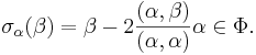

In view of property 3, the integrality condition is equivalent to stating that β and its reflection σα(β) differ by an integer multiple of α. Note that the operator
defined by property 4 is not an inner product. It is not necessarily symmetric and is linear only in the first argument.
The integrality condition also means that the ratio of the lengths (magnitudes) of any two roots cannot be 2 or greater, since otherwise either the projection of the shorter root onto the longer root will be less than half as long as the longer root, or the shorter root will be exactly half the longer root or its negative.
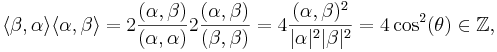
The cosine of the angle between two roots is constrained to be a half-integral multiple of a square root of an integer:
These values can only be  , corresponding to angles of 30°, 45°, 60°, 90°, 120°, 135°, 150°.
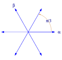
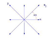
The rank of a root system Φ is the dimension of V. Two root systems may be combined by regarding the Euclidean spaces they span as mutually orthogonal subspaces of a common Euclidean space. A root system which does not arise from such a combination, such as the systems A2, B2, and G2 pictured below, is said to be irreducible.
Two irreducible root systems (E1,Φ1) and (E2,Φ2) are considered to be the same if there is an invertible linear transformation E1→E2 which sends Φ1 to Φ2.
The group of isometries of V generated by reflections through hyperplanes associated to the roots of Φ is called the Weyl group of Φ. As it acts faithfully on the finite set Φ, the Weyl group is always finite.
The root lattice of a root system Φ is the Z-submodule of V generated by Φ. It is a lattice in V.
Rank 1 and rank 2 examples
There is only one root system of rank 1, consisting of two nonzero vectors {α, −α}. This root system is called A1.
In rank 2 there are four possibilities, corresponding to σα(β) = β + nα, where n = 0, 1, 2, 3.
 |
 |
| Root system A1×A1 | Root system A2 |
 |
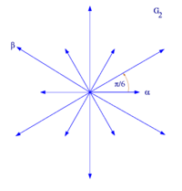 |
| Root system B2 | Root system G2 |
Whenever Φ is a root system in V and W is a subspace of V spanned by Ψ=Φ∩W, then Ψ is a root system in W. Thus, our exhaustive list of root systems of rank 2 shows the geometric possibilities for any two roots chosen from a root system of arbitrary rank. In particular, two such roots meet at an angle of 0, 30, 45, 60, 90, 120, 135, 150, or 180 degrees.
Positive roots and simple roots
Given a root system Φ we can always choose (in many ways) a set of positive roots. This is a subset  of Φ such that
- for each root
 exactly one of the roots
  is contained in
 - For any
 such that
  is a root,
 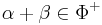 .
.
If a set of positive roots is chosen, elements of ( ) are called negative roots.
An element of is called indecomposable or simple if it cannot be written as the sum of two elements of . The set  of simple roots is a basis of
  with the property that every vector in
  is a linear combination of elements of with all coefficients non-negative, or all coefficients non-positive.
It can be shown that for each choice of positive roots there exists a unique set of simple roots so that the positive roots are exactly those roots that can be expressed as a combination of simple roots with non-negative coefficients.
Dual root system and coroots
- See also: Langlands dual group
If Φ is a root system in V, the coroot αV of a root α is defined by
The set of coroots roots also forms a root system ΦV in V, called the dual root system (or sometimes inverse root system). By definition, αV V = α, so that Φ is the dual root system of ΦV. The lattice in V spanned by ΦV is called the coroot lattice. Both Φ and ΦV have the same Weyl group W and, for s in W,
If Δ is a set of simple roots for Φ, then ΔV is a set of simple roots for ΦV.
Classification of root systems by Dynkin diagrams
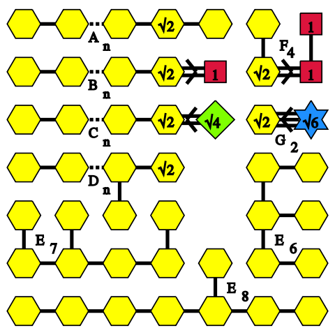
Irreducible root systems correspond to certain graphs, the Dynkin diagrams named after Eugene Dynkin. The classification of these graphs is a simple matter of combinatorics, and induces a classification of irreducible root systems.
Given a root system, select a set Δ of simple roots as in the preceding section. The vertices of the associated Dynkin diagram correspond to vectors in Δ. An edge is drawn between each non-orthogonal pair of vectors; it is an undirected single edge if they make an angle of 120 degrees, a directed double edge if they make an angle of 135 degrees, and a directed triple edge if they make an angle of 150 degrees. The term "directed edge" means that double and triple edges are marked with an angle sign pointing toward the shorter vector.
Although a given root system has more than one possible set of simple roots, the Weyl group acts transitively on such choices. Consequently, the Dynkin diagram is independent of the choice of simple roots; it is determined by the root system itself. Conversely, given two root systems with the same Dynkin diagram, one can match up roots, starting with the roots in the base, and show that the systems are in fact the same.
Thus the problem of classifying root systems reduces to the problem of classifying possible Dynkin diagrams. The problem of classifying irreducible root systems reduces to the problem of classifying connected Dynkin diagrams. Dynkin diagrams encode the inner product on E in terms of the basis Δ, and the condition that this inner product must be positive definite turns out to be all that is needed to get the desired classification.
The actual connected diagrams are as follows. The subscripts indicate the number of vertices in the diagram (and hence the rank of the corresponding irreducible root system).

Properties of the irreducible root systems
|
 |
 |
I | D |  |
|---|---|---|---|---|---|
| An (n≥1) | n(n+1) | n+1 | (n+1)! | ||
| Bn (n≥2) | 2n2 | 2n | 2 | 2 | 2n n! |
| Cn (n≥3) | 2n2 | 2n(n−1) | 2 | 2 | 2n n! |
| Dn (n≥4) | 2n(n−1) | 4 | 2n−1 n! | ||
| E6 | 72 | 3 | 51840 | ||
| E7 | 126 | 2 | 2903040 | ||
| E8 | 240 | 1 | 696729600 | ||
| F4 | 48 | 24 | 4 | 1 | 1152 |
| G2 | 12 | 6 | 3 | 1 | 12 |
Irreducible root systems are named according to their corresponding connected Dynkin diagrams. There are four infinite families (An, Bn, Cn, and Dn, called the classical root systems) and five exceptional cases (the exceptional root systems). The subscript indicates the rank of the root system.
In an irreducible root system there can be most two values for the length (α, α)½, corresponding to short and long roots. If all roots have the same length they are taken to be long by definition and the root system is said to be simply laced; this occurs in the cases A, D and E. Any two roots of the same length lie in the same orbit of the Weyl group. In the non-simply laced cases B, C, G and F, the root lattice is spanned by the short roots and the long roots span a sublattice, invariant under the Weyl group, equal to r2/2 times the coroot lattice, where r is the length of a long root.
In the table to the right, denotes the number of short roots, I denotes the index in the root lattice of the sublattice generated by long roots, D denotes the determinant of the Cartan matrix, and denotes the order of the Weyl group.
Explicit construction of the irreducible root systems
An
| 1 | -1 | 0 | 0 |
| 0 | 1 | -1 | 0 |
| 0 | 0 | 1 | -1 |
Let V be the subspace of Rn+1 for which the coordinates sum to 0, and let Φ be the set of vectors in V of length √2 and which are integer vectors, i.e. have integer coordinates in Rn+1. Such a vector must have all but two coordinates equal to 0, one coordinate equal to 1, and one equal to −1, so there are n2 + n roots in all. One choice of simple roots expressed in the standard basis is: αi = ei - ei+1, for 1 ≤ i ≤ n.
The reflection σi through the hyperplane perpendicular to αi is the same as permutation of the adjacent ith and i+1th coordinates. Such transpositions generate the full permutation group. For adjacent simple roots, σi(αi+1) = αi+1 + αi = σi+1(αi) = αi + αi+1, that is, reflection is equivalent to adding a multiple of 1; but reflection of a simple root perpendicular to a nonadjacent simple root leaves it unchanged, differing by a multiple of 0.
Bn
| 1 | -1 | 0 | 0 |
| 0 | 1 | -1 | 0 |
| 0 | 0 | 1 | -1 |
| 0 | 0 | 0 | 1 |
Let V=Rn, and let Φ consist of all integer vectors in V of length 1 or √2. The total number of roots is 2n2. One choice of simple roots is: αi = ei - ei+1, for 1 ≤ i ≤ n-1 (the above choice of simple roots for An-1), and the shorter root αn = en.
The reflection σn through the hyperplane perpendicular to the short root αn is of course simply negation of the nth coordinate. For the long simple root αn-1, σn-1(αn) = αn + αn-1, but for reflection perpendicular to the short root, σn(αn-1) = αn-1 + 2αn, a difference by a multiple of 2 instead of 1.
B1 is isomorphic to A1 via scaling by √2, and is therefore not a distinct root system.
Cn
| 1 | -1 | 0 | 0 |
| 0 | 1 | -1 | 0 |
| 0 | 0 | 1 | -1 |
| 0 | 0 | 0 | 2 |
Let V=Rn, and let Φ consist of all integer vectors in V of length √2 together with all vectors of the form 2λ, where λ is an integer vector of length 1. The total number of roots is 2n2. One choice of simple roots is: αi = ei - ei+1, for 1 ≤ i ≤ n-1 (the above choice of simple roots for An-1), and the longer root αn = 2en. The reflection σn(αn-1) = αn-1 + αn, but σn-1(αn) = αn + 2αn-1.
C2 is isomorphic to B2 via scaling by √2 and a 45 degree rotation, and is therefore not a distinct root system.
Dn
| 1 | -1 | 0 | 0 |
| 0 | 1 | -1 | 0 |
| 0 | 0 | 1 | -1 |
| 0 | 0 | 1 | 1 |
Let V=Rn, and let Φ consist of all integer vectors in V of length √2. The total number of roots is 2n(n−1). One choice of simple roots is: αi = ei - ei+1, for 1 ≤ i < n (the above choice of simple roots for An-1) plus αn = en + en-1.
Reflection through the hyperplane perpendicular to αn is the same as transposing and negating the adjacent nth and n-1th coordinates. Any simple root and its reflection perpendicular to another simple root differ by a multiple of 0 or 1 of the second root, not by any greater multiple.
D3 reduces to A3, and is therefore not a distinct root system.
D4 has additional symmetry called triality.
E8, E7, E6
The E8 lattice can be defined as explicitly by the set of points Γ8 ⊂ R8 such that:
- all the coordinates are integers or all the coordinates are half-integers (a mixture of integers and half-integers is not allowed), and
- the sum of the eight coordinates is an even integer.
Let the E8 root system be the set of vectors of length √2 in Γ8, that is: (α ∈ Z8 ∪ (Z+½)8: |α|2 = ∑αi2 = 2, ∑αi ∈ 2Z).
Then let E7 be the intersection of E8 with the hyperplane of vectors perpendicular to a fixed root in E8, and let E6 the intersection of E7 with the hyperplane of vectors perpendicular to a fixed root in E7. The root systems E6, E7, and E8 have 72, 126, and 240 roots respectively. If we continue to delete roots and reduce dimension, E5 reduces to D5, and E4 reduces to A4, so no more distinct root systems are found.
| 1 | -1 | 0 | 0 | 0 | 0 | 0 | 0 |
| 0 | 1 | -1 | 0 | 0 | 0 | 0 | 0 |
| 0 | 0 | 1 | -1 | 0 | 0 | 0 | 0 |
| 0 | 0 | 0 | 1 | -1 | 0 | 0 | 0 |
| 0 | 0 | 0 | 0 | 1 | -1 | 0 | 0 |
| 0 | 0 | 0 | 0 | 0 | 1 | -1 | 0 |
| 0 | 0 | 0 | 0 | 0 | 1 | 1 | 0 |
| ½ | ½ | ½ | ½ | ½ | ½ | ½ | ½ |
An alternative description of the E8 lattice which is sometimes convenient is the set of all points in Γ′8 ⊂ R8 such that
- all the coordinates are integers and the sum of the coordinates is even, or
- all the coordinates are half-integers and the sum of the coordinates is odd.
The lattices Γ8 and Γ′8 are isomorphic and one may pass from one to the other by changing the signs of any odd number of coordinates. The lattice Γ8 is sometimes called the even coordinate system for E8 while the lattice Γ′8 is called the odd coordinate system.
One choice of simple roots for E8 in the even coordinate system is: αi = ei - ei+1, for 1 ≤ i ≤ 6 and α7 = e7 + e6 (the above choice of simple roots for D7) along with α8 = β0 =  = (½,½,½,½,½,½,½,½).
| 1 | -1 | 0 | 0 | 0 | 0 | 0 | 0 |
| 0 | 1 | -1 | 0 | 0 | 0 | 0 | 0 |
| 0 | 0 | 1 | -1 | 0 | 0 | 0 | 0 |
| 0 | 0 | 0 | 1 | -1 | 0 | 0 | 0 |
| 0 | 0 | 0 | 0 | 1 | -1 | 0 | 0 |
| 0 | 0 | 0 | 0 | 0 | 1 | -1 | 0 |
| 0 | 0 | 0 | 0 | 0 | 0 | 1 | -1 |
| -½ | -½ | -½ | -½ | -½ | ½ | ½ | ½ |
One choice of simple roots for E8 in the odd coordinate system is: αi = ei - ei+1, for 1 ≤ i ≤ 7 (the above choice of simple roots for A7) along with α8 = β5, where βj =  . (Using β3 would give an isomorphic result. Using β1,7 or β2,6 would simply give A8 or D8. As for β4, its coordinates sum to 0, and the same is true for α1...7, so they span only the 7-dimensional subspace for which the coordinates sum to 0; in fact -2β4 = has coordinates (1,2,3,4,3,2,1) in the basis (αi).)
Deleting α1 and then α2 gives sets of simple roots for E7 and E6. Since perpendicularity to α1 means that the first two coordinates are equal, E7 is then the subspace of E8 where the first two coordinates are equal, and similarly E6 is the subspace of E8 where the first three coordinates are equal. This facilitates explicit definitions of E7 and E6 as:
E7 = (α ∈ Z7 ∪ (Z+½)7: ∑αi2 + α12 = 2, ∑αi + α1 ∈ 2Z), E6 = (α ∈ Z6 ∪ (Z+½)6: ∑αi2 + 2α12 = 2, ∑αi + 2α1 ∈ 2Z)
F4
| 1 | -1 | 0 | 0 |
| 0 | 1 | -1 | 0 |
| 0 | 0 | 1 | 0 |
| -½ | -½ | -½ | -½ |
For F4, let V=R4, and let Φ denote the set of vectors α of length 1 or √2 such that the coordinates of 2α are all integers and are either all even or all odd. There are 48 roots in this system. One choice of simple roots is: the choice of simple roots given above for B3, plus α4 =  .
.
G2
| 1 | -1 | 0 |
| -1 | 2 | -1 |
G2 has 12 roots, which form the vertices of a hexagram. See the picture above.
One choice of simple roots is: (α1, β=α2-α1) where αi = ei - ei+1 for i = 1, 2 is the above choice of simple roots for A2.
Root systems and Lie theory
Irreducible root systems classify a number of related objects in Lie theory, notably:
- Simple complex Lie algebras
- Simple complex Lie groups
- Simply connected complex Lie groups which are simple modulo centers
- Simple compact Lie groups
In each case, the roots are non-zero weights of the adjoint representation.
In the case of a simply connected connected simple compact Lie group G with maximal torus T, the root lattice can naturally be identified with Hom(T, T) and the coroot lattice with Hom(T, T); see Adams (1983).
Extended and affine Dynkin diagrams
-
For more details on this topic, see Coxeter group#Affine_Weyl_groups.
There are extensions of Dynkin diagrams, namely extended Dynkin diagrams and affine Dynkin diagrams.
Extended Dynkin diagrams are denoted with a tilde, as in  .
.
Affine Dynkin diagrams describe Cartan matrices of affine Lie algebras.
See also
- Weyl group, Coxeter group
- Coxeter matrix
- ADE classification
- root datum
- Coxeter-Dynkin diagram
References
- Adams, J.F. (1983), Lectures on Lie groups, University of Chicago Press, ISBN 0226005305
- Bourbaki, Nicolas (2002), Lie groups and Lie algebras, Chapters 4-6 (translated from the 1968 French original by Andrew Pressley), Elements of Mathematics, Springer-Verlag, ISBN 3-540-42650-7. The classic reference for root systems.
Further reading
- Dynkin, E. B. The structure of semi-simple algebras. (Russian) Uspehi Matem. Nauk (N.S.) 2, (1947). no. 4(20), 59--127.