Recurrence relation
- "Difference equation" redirects here. It should not be confused with a differential equation.
In mathematics, a recurrence relation is an equation that defines a sequence recursively: each term of the sequence is defined as a function of the preceding terms.
A difference equation is a specific type of recurrence relation.
An example of a recurrence relation is the logistic map:
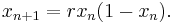
Some simply defined recurrence relations can have very complex (chaotic) behaviours and are sometimes studied by physicists and mathematicians in a field of mathematics known as nonlinear analysis.
Solving a recurrence relation means obtaining a closed-form solution: a non-recursive function of n.
Linear homogeneous recurrence relations with constant coefficients
The term linear means that each term of the sequence is defined as a linear function of the preceding terms. The order of a linear recurrence relation is the number of preceding terms required by the definition—so the relation  is of order two, because there must be at least two preceding terms (whether they are both used or not).
The general form of a linear recurrence relation of order  is as follows:

where  and
and  (for all
  ) are allowed to depend on
  , but
, but  (for all ) is not. If is independent of (for all ), then the recurrence relation is said to have constant coefficients. Additionally, if
  then the recurrence relation is homogeneous; such a sequence is also called a linear recursive sequence or LRS.
The linear recurrence, together with seed values (initial conditions) for  , determines the sequence uniquely.
Example: Fibonacci numbers
The Fibonacci numbers are defined using the linear recurrence relation

with seed values:


The sequence of Fibonacci numbers begins:
- 1, 1, 2, 3, 5, 8, 13, 21, 34, 55, 89 ...
It can be solved via the matrix solution described below, yielding the closed form expression.
Solving via linear algebra
Given an LRS, one can write down its companion matrix, then put it in Jordan normal form (which is diagonal if the eigenvalues are distinct). Expressing the seed in terms of the eigenbasis, say
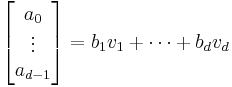
yields
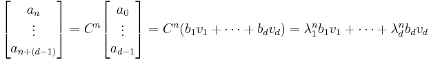
which is a closed form expression (expand on the first coordinate to obtain a closed form expression for  ).
).
If the companion matrix is not diagonalizable, then the resulting expression is more complicated, but conceptually the same.
Solving generally
Solutions to recurrence relations are found by systematic means, often by using generating functions (formal power series) or by noticing the fact that rn is a solution for particular values of r.
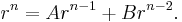
Consider, for example, a recurrence relation of the form
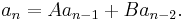
(see also Fibonacci family).
Suppose that it has a solution of the form an = rn. Substituting this guess in the recurrence relation, we find:
Dividing through by rn − 2, we get
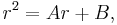

This is known as the characteristic equation of the recurrence relation. Solve for r to obtain the two roots λ1, λ2, and if these roots are distinct, we have the solution
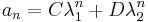
while if they are identical (when A2 + 4B = 0), we have
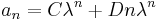
where constants C and D can be found from the "side conditions" that are often given as a0 = a, a1 = b.
Different solutions are obtained depending on the nature of the roots of the characteristic equation.
Solving with z-transforms
Certain difference equations, in particular Linear constant coefficient difference equations, can be solved using z-transforms. The z-transforms are a class of integral transforms that lead to more convenient algebraic manipulations and more straightforward solutions. There are cases in which obtaining a direct solution would be all but impossible, yet solving the problem via a thoughtfully chosen integral transform is straightforward.
Theorem
Given a linear homogeneous recurrence relation with constant coefficients of order , let  be the characteristic polynomial (also "auxiliary polynomial")

such that each corresponds to each in the original recurrence relation (see the general form above). Suppose  is a root of having multiplicity
  . This is to say that
  divides . The following two properties hold:
- Each of the sequences
 satisfies the recurrence relation.
 - Any sequence satisfying the recurrence relation can be written uniquely as a linear combination of solutions constructed in part 1 as varies over all distinct roots of .
As a result of this theorem a linear homogeneous recurrence relation with constant coefficients can be solved in the following manner:
- Find the characteristic polynomial .
- Find the roots of counting multiplicity.
- Write as a linear combination of all the roots (counting multiplicity as shown in the theorem above) with unknown coefficients
 .
.

-
- This is the general solution to the original recurrence relation.
-
- (Note:
 is the multiplicity of
  )
)
- (Note:
- 4. Equate each
 from part 3 (plugging in
  into the general solution of the recurrence relation) with the known values from the original recurrence relation. Note, however, that the values from the original recurrence relation used do not have to be contiguous, just of them are needed (i.e. for an original linear homogeneous recurrence relation of order 3 one could use the values
  ). This process will produce a linear system of equations with unknowns. Solving these equations for the unknown coefficients
  of the general solution and plugging these values back into the general solution will produce the particular solution to the original recurrence relation that fits the original recurrence relation's initial conditions (as well as all subsequent values
  of the original recurrence relation).
Interestingly, the method for solving linear differential equations is similar to the method above — the "intelligent guess" for linear differential equations with constant coefficients is  where is a complex number that is determined by substituting the guess into the differential equation.
This is not a coincidence. If you consider the Taylor series of the solution to a linear differential equation:
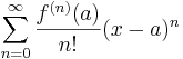
you see that the coefficients of the series are given by the n-th derivative of f(x) evaluated at the point a. The differential equation provides a linear difference equation relating these coefficients.
This equivalence can be used to quickly solve for the recurrence relationship for the coefficients in the power series solution of a linear differential equation.
The rule of thumb (for equations in which the polynomial multiplying the first term is non-zero at zero) is that:
![y^{[k]} \to f[n+k]](/2009-wikipedia_en_wp1-0.7_2009-05/I/19d7803b0166b65a77fe2970279cc30e.png)
and more generally
![x^m*y^{[k]} \to n(n-1)(n-m+1)f[n+k-m]](/2009-wikipedia_en_wp1-0.7_2009-05/I/0acc80c8056f394455dfa25158339a69.png)
Example: The recurrence relationship for the Taylor series coefficients of the equation:
![(x^2 + 3x -4)y^{[3]} -(3x+1)y^{[2]} + 2y = 0\,](/2009-wikipedia_en_wp1-0.7_2009-05/I/ee3fd58586a3e67e5a34f5a4dde4df45.png)
is given by
![n(n-1)f[n+1] + 3nf[n+2] -4f[n+3] -3nf[n+1] -f[n+2]+ 2f[n] = 0\,](/2009-wikipedia_en_wp1-0.7_2009-05/I/b82d03a5c967d1e72b51142b7a0dd577.png)
or
![-4f[n+3] +2nf[n+2] + n(n-4)f[n+1] +2f[n] = 0.\,](/2009-wikipedia_en_wp1-0.7_2009-05/I/10b618dc04c186e3594fdead26c020c1.png)
This example shows how problems generally solved using the power series solution method taught in normal differential equation classes can be solved in a much easier way.
Example: The differential equation
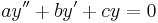
has solution

The conversion of the differential equation to a difference equation of the Taylor coefficients is
![af[n + 2] + bf[n + 1] + cf[n] = 0\,](/2009-wikipedia_en_wp1-0.7_2009-05/I/8c0dd7e2ec42ce6d6e65af6fe0aeb9f1.png) .
.
It is easy to see that the nth derivative of eax evaluated at 0 is an
General linear homogeneous recurrence relations
Many linear homogeneous recurrence relations may be solved by means of the hypergeometric series. Special cases of these lead to recurrence relations for the orthogonal polynomials, and many special functions. For example, the solution to
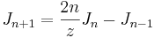
is given by
 ,
,
the Bessel function, while

is solved by
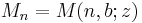
the confluent hypergeometric series.
Solving non-homogeneous recurrence relations
If the recurrence is inhomogeneous, a particular solution can be found by the method of undetermined coefficients and the solution is the sum of the solution of the homogeneous and the particular solutions. Another method to solve an inhomogeneous recurrence is the method of symbolic differentiation. For example, consider the following recurrence:

This is an inhomogeneous recurrence. If we substitute  , we obtain the recurrence
Subtracting the original recurrence from this equation yields

or equivalently
This is a homogeneous recurrence which can be solved by the methods explained above. In general, if a linear recurrence has the form

where  are constant coefficients and
  is the inhomogeneity, then if is a polynomial with degree
  , then this inhomogeneous recurrence can be reduced to a homogeneous recurrence by applying the method of symbolic differentiation times.
Relationship to difference equations
Given a sequence  of real numbers: the first difference
  is defined as
 .
.
The second difference  is defined as
 ,
,
which can be simplified to
 .
.
More generally: the kth difference  is defined as
 .
.
A difference equation is an equation composed of and its kth differences.
Every recurrence relation can be formulated as a difference equation. Conversely, every difference equation can be formulated as a recurrence relation. Some authors thus use the two terms interchangeably. For example, the difference equation
is equivalent to the recurrence relation
See time scale calculus for a unification of the theory of difference equations with that of differential equations.
Relationship to differential equations
When solving an ordinary differential equation numerically, one typically encounters a recurrence relation. For example, when solving the initial value problem

with Euler's method and a step size h, one calculates the values

by the recurrence
Systems of linear first order differential equations can be discretized exactly analytically using the methods shown in the discretization article.
Application to biology
Some of the best-known difference equations have their origins in the attempt to model population dynamics. For example, the Fibonacci numbers were once used as a model for the growth of a rabbit population.
The logistic map is used either directly to model population growth, or as a starting point for more detailed models. In this context, coupled difference equations are often used to model the interaction of two or more populations. For example, the Nicholson-Bailey model for a host-parasite interaction is given by
 ,
,
with  representing the hosts, and
  the parasites, at time
  .
.
Integrodifference equations are a form of recurrence relation important to spatial ecology. These and other difference equations are particularly suited to modeling univoltine populations.
See also
- Hypergeometric series
- Orthogonal polynomial
- Recursion
- Recursion (computer science)
- Lagged Fibonacci generator
- Master theorem
- Circle points segments proof
- Continued fraction
- Time scale calculus
- Integrodifference equation
References
- Thomas H. Cormen, Charles E. Leiserson, Ronald L. Rivest, and Clifford Stein. Introduction to Algorithms, Second Edition. MIT Press and McGraw-Hill, 1990. ISBN 0-262-03293-7. Chapter 4: Recurrences, pp.62–90.
- Ian Jacques. Mathematics for Economics and Business, Fifth Edition. Prentice Hall, 2006. ISBN 0-273-70195-9. Chapter 9.1: Difference Equations, pp.551–568.
- Paul M. Batchelder, An introduction to linear difference equations, Dover Publications, 1967.
- Kenneth S. Miller, Linear difference equations. W.A. Benjamin, 1968.
- Difference and Functional Equations: Exact Solutions at EqWorld - The World of Mathematical Equations.
- Difference and Functional Equations: Methods at EqWorld - The World of Mathematical Equations.
- Applied Econometric time series, Second Edition. Walter Enders.
External links
- Eric W. Weisstein, Recurrence Equation at MathWorld.
- Homogeneous Difference Equations by John H. Mathews
- Online Solver for Linear Recurrence Sequences: provides closed form of linear recurrence sequences
- Introductory Discrete Mathematics