Projective space
In mathematics a projective space is a set of elements constructed from a vector space such that a distinct element of the projective space consists of all non-zero vectors which are equal up to a multiplication by a non-zero scalar. A formal definition of a projective space can be formulated in several ways, and can also be made more abstract, see below. The projective space generated from a particular vector space V is often denoted P(V). The cases when V=R2 or V=R3 are the projective line and the projective plane, respectively.
The idea of a projective space relates to perspective, more precisely to the way an eye or a camera projects a 3D scene to a 2D image. All points which lie on a projection line (i.e. a "line-of-sight"), intersecting with the focal point of the camera, are projected onto a common image point. In this case the vector space is R3 with the camera focal point at the origin and the projective space corresponds to the image points.
Projective spaces can be studied as a separate field in mathematics, but are also used in various applied fields, geometry in particular. Geometric objects, such as points, lines, or planes, can be given a representation as elements in projective spaces based on homogeneous coordinates. As a result, various relations between these objects can be described in simpler way than is possible without homogeneous coordinates. Furthermore, various statements in geometry can be made more consistent and without exceptions. For example, in the standard geometry for the plane two lines always intersect at a point except when the lines are parallel. In a projective representation of lines and points, however, such an intersection point exists even for parallel lines, and it can be computed in the same way as other intersection points.
Other mathematical fields where projective spaces play a significant role are topology, the theory of Lie groups and algebraic groups, and their representation theories.
Contents |
Introduction

As outlined above, projective space is a geometric object formalizing statements like "Parallel lines intersect at infinity". For concreteness, we will give the construction of the real projective plane Rℙ2 in some detail. There are three equivalent definitions: First, the set of all lines in (real 3-)space R3 passing through the origin (0, 0, 0). Every such line meets the sphere of radius one centered in the origin exactly twice, say in P = (x, y, z) and its antipodal point (-x, -y, -z). Thus Rℙ2 can also be described to be the points on the sphere S2, where every point P and its antipodal point are not distinguished. For example, the point (1, 0, 0) (red point in the image) is identified with (-1, 0, 0) (light red point), etc. Finally, yet another equivalent definition is the set of equivalence classes of R3\(0, 0, 0), i.e. 3-space without the origin, where two points P = (x, y, z) and Pˈ = (xˈ, yˈ, zˈ) are equivalent iff there is a nonzero real number λ such that P = λ·Pˈ, i.e. x = λxˈ, y = λyˈ, z = λzˈ. The usual way to write an element of the projective plane, i.e. the equivalence class corresponding to an honest point (x, y, z) in R3, is
- [x : y : z]
This goes under the name of homogenous coordinates.
Notice that any point [x : y : z] with z ≠ 0 is equivalent to [x/z : y/z : 1]. So there are two disjoint subsets of the projective plane: that consisting of the points [x : y : z] = [x/z : y/z : 1] for z ≠ 0, and that consisting of the remaining points [x : y : 0]. The latter set can be subdivided similarly into two disjoint subsets, with points [x/y : 1 : 0] and [x : 0 : 0]. In the last case, x is necessarily nonzero, because the origin was not part of Rℙ2. Thus the point is equivalent to [1 : 0 : 0]. Geometrically, the first subset, which is isomorphic (not only as a set, but also as a manifold, as will be seen later) to R2, is in the image the yellow upper hemisphere (without the equator), or equivalently the lower hemisphere. The second subset, isomorphic to R1, corresponds to the green line (without the two marked points), or, again, equivalently the light green line. Finally we have the red point or the equivalent light red point. We thus have a disjoint decomposition
- Rℙ2 = R2 ⊔ R1 ⊔ point.
Intuitively already clear, and made precise below, R1 ⊔ point is itself the real projective line Rℙ1. Considered as a subset of Rℙ2, it is called line at infinity, whereas R2 ⊂ Rℙ2 is called affine plane, i.e. just the usual plane.
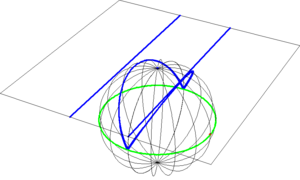
The next objective is make precise the saying: "parallel lines meet at infinity". A natural bijection between the plane z = 1 (which meets the sphere at the north pole N = (0, 0, 1)) and the affine plane (i.e. the upper hemisphere) inside projective plane is accomplished by the stereographic projection, i.e. any point P on this plane is mapped to the intersection point of the line through the origin and P and the sphere. Therefore two lines L1 and L2 (blue) in the plane are mapped to what looks like great circles (antipodal points are identified, though). Great circles intersect precisely in two antipodal points, which are identified in the projective plane, i.e. any two lines have exactly one intersection point inside Rℙ2. This phenomenon is axiomatized and studied in projective geometry.
Definition of projective space
Real projective space is defined by
- Rℙn := (Rn+1 \ {0})/~,
with the equivalence relation (x0, ..., xn) ~ (λx0, ..., λxn), where λ is an arbitrary non-zero real number. Equivalently, it is the set of all lines in Rn+1 passing through the origin 0 := (0, ..., 0).
Instead of R, one may take any arbitrary field, or even a division ring k. For the complex numbers or the quaternions, one obtains the complex projective space Cℙn and quaternionic projective space Hℙn. In algebraic geometry the usual notation for projective space is ℙnk.
If n is one or two, it is also called projective line or projective plane, respectively. The complex projective line is also called Riemann sphere.
As in the above special case, the notation (so-called homogenous coordinates) for a point in projective space is
- [x0 : ... : xn].
Slightly more general, for a vector space V (over some field k, or, more generally a module V over some division ring), ℙ(V) is defined to be (V\{0})/~, where two non-zero vectors v1, v2 in V are equivalent if they differ by a non-zero scalar λ, i.e. v1 = λ·v2. The vector space need not be finite-dimensional, which is used, for example, in the theory of projective Hilbert spaces.
In the theory of Alexander Grothendieck, especially in the construction of projective bundles, there are reasons for applying the construction outlined above rather to the dual space V*, the reasons being that we would like to associate a projective space to every scheme Y and every quasi-coherent sheaf E over Y, not just the locally free ones. See EGAII, Chap. II, par. 4 for more details.
Projective space as a manifold

The above definition of projective space gives a set. For purposes of differential geometry, which deals with manifolds, it is useful to endow this set with a (real or complex) manifold structure.
Namely consider the following subsets: Ui = {[x0: ...: xn], xi ≠ 0}, i = 0, ..., n. By the definition of projective space, their union is the whole projective space. Further, Ui is in bijection to Rn (or Cn) via
![[x_0: ...: x_n] \mapsto (\frac{x_0}{x_i}, ..., \hat{\frac{x_i}{x_i}}, ..., \frac{x_n}{x_i})](/2009-wikipedia_en_wp1-0.7_2009-05/I/050b3075f6116ce859ea553d04a3aea3.png)
![[y_0: ...: y_{i-1}: 1: y_{i+1}: ... y_n] \leftarrow (y_0, ..., \hat{y_i}, ... y_n)](/2009-wikipedia_en_wp1-0.7_2009-05/I/099f2dfdd807af1ab98045e1fc32a6a0.png)
(the hat means that the i-th entry is missing).
The example image shows Rℙ1. (Antipodal points are identified in Rℙ1, though). It is covered by two copies of the real line R, each of which covers the projective line except one point, which is "the" (or a) point at infinity.
We first define a topology on projective space by declaring that these maps shall be homeomorphisms, that is, an subset of Ui is open iff its image under the above isomorphism is an open subset (in the usual sense) of Rn. An arbitrary subset A of Rℙn is open if all intersections A ∩ Ui are open. This defines a topological space.
The manifold structure is given by the above maps, too.

Another way to think about the projective line is the following: take two copies of the affine line with coordinates x and y, respectively, and glue them together along the subsets x ≠ 0 and y ≠ 0 via the maps
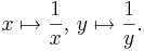
The resulting manifold is the projective line. The charts given by this construction are the same as the ones above. Similar presentations exist for higher-dimensional projective spaces.
The above decomposition in disjoint subsets reads in this generality:
- Rℙn = Rn ⊔ Rn-1 ⊔ ... ⊔ R1 ⊔ R0,
this so-called cell-decomposition can be used to calculate the singular cohomology of projective space.
All of the above holds for complex projective space, too. The complex projective line Cℙ1 is an example of a Riemann surface.
The covering by the above open subsets also shows that projective space is an algebraic variety (or scheme), it is covered by n + 1 affine n-spaces. The construction of projective scheme is an instance of the Proj construction.
Why the projective space is "better" than the affine space

There are a number of mathematically deeply meaningful advantages of the projective space against affine space (e.g. RPn vs. Rn). For these reasons it is important to know when a given manifold or variety is projective, i.e. embeds into (is a closed subset of) projective space. (Very) ample line bundles are designed to tackle this question.
- Projective space is a compact topological space, affine space is not. Therefore, Liouville's theorem applies to show that every holomorphic function on CPn is constant. Another consequence is, for example, that integrating functions or differential forms on Pn does not cause convergence issues.
- On a projective complex manifold X, cohomology groups of coherent sheaves F
- H∗(X, F)
 , the zero-th cohomology of the sheaf of holomorphic functions). In the parlance of algebraic geometry, projective space is proper. The above results hold in this context, too.
 - For complex projective space, every complex submanifold X ⊂ CPn (i.e., a manifold cut out by holomorphic equations) is necessarily an algebraic variety (i.e., given by polynomial equations). This is Chow's theorem, it allows the direct use of algebraic-geometric methods for these ad hoc analytically defined objects.
- As outlined above, lines in P2 or more generally hyperplanes in Pn always do intersect. This extends to non-linear objects, as well: appropriately defining the degree of an algebraic curve, which is roughly the degree of the polynomials needed to define the curve (see Hilbert polynomial), it is true (over an algebraically closed field k) that any two projective curves C1 and C2 ⊂ Pkn of degree e and f intersect in exactly e·f points, counting them with multiplicities (see Bézout's theorem). This is applied, for example, in defining a group structure on the points of an elliptic curve, like y2 = x3−x+1. The degree of an elliptic curve is 3. Consider the line x = 1, which intersects the curve (inside affine space) exactly twice, namely in (1, 1) and (1, −1). However, inside P2, the projective closure of the curve is given by the homogeneous equation
- y2·z = x3−x·z2+z3,
- Any projective group variety, i.e. a projective variety, whose points form an abstract group, is necessarily an abelian variety, i.e. the group operation is commutative. Elliptic curves are examples for abelian varieties. The commutativity fails for non-projective group varieties, as the example GLn(k) (the general linear group) shows.
Axiomatic characterization of projective space
There is an alternative axiomatic approach to projective spaces defining them as an incidence structure with certain properties. This approach does not rely on the construction over vector spaces (ℙ(V)) and is in particular popular in the fields of finite geometry and combinatorics. For a projective space of dimension ≧3 it can be shown that it is isomorphic to ℙ(V) for some V. However for projective spaces of dimension 2 (projective planes) this is not true, i.e. there exist projective planes which are not isomorphic to ℙ(V) for any V, so the ℙ(V) construction does not describe all projective planes. A projective plane that is constructed over a Moulton plane is an example of such a projective plane, that cannot be described through ℙ(V) for some V.
Morphisms
Injective linear maps T ∈ L(V,W) between two vector spaces V and W over the same field k induce mappings of the corresponding projective spaces via
![\mathbb P(V) \rightarrow \mathbb P(W), [\mathbf{v}]\mapsto [T(\mathbf{v})],](/2009-wikipedia_en_wp1-0.7_2009-05/I/84f2bbb38474ea660f1d05e1fcbb5a74.png)
where v is a non-zero element of V and [...] denotes the equivalence classes of a vector under the defining identification of the respective projective spaces. Since members of the equivalence class differ by a scalar factor, and linear maps preserve scalar factors, this induced map is well-defined. (If T is not injective, it will have a null space larger than {0}; in this case the meaning of the class of T(v) is problematic if v is non-zero and in the null space. In this case one obtains a so-called rational map, see also birational geometry).
Two linear maps S and T in L(V,W) induce the same map between ℙ(V) and ℙ(W) iff they differ by a scalar multiple of the identity, that is if T=λS for some λ ≠ 0. Thus if one identifies the scalar multiples of the identity map with the underlying field, the set of k-linear morphisms from ℙ(V) to ℙ(W) is simply ℙ(L(V,W)).
The automorphisms ℙ(V) → ℙ(V) can be described more concretely. (We deal only with automorphisms preserving the base field k). Using the notion of sheaves generated by global sections, it can be shown that any algebraic (not necessarily linear) automorphism has to be linear, i.e. coming from a (linear) automorphism of the vector space V. They form the group GL(V). By identifying maps which differ by a scalar, one concludes
- Aut(ℙ(V)) = Aut(V)/k∗ = GL(V)/k∗ =: PGL(V),
the quotient group of GL(V) modulo the matrices which are scalar multiples of the identity. (These matrices form the center of Aut(V)). The groups PGL are called projective linear groups. The automorphisms of the complex projective line Cℙ1 are called Möbius transformations.
Generalizations
The projective space, being the "space" of all one-dimensional linear subspaces of a given vector space V is generalized to Grassmannian manifold, which is parametrizing higher-dimensional subspaces (of some fixed dimension) of V. More generally flag manifold is the space of flags, i.e. chains of linear subspaces of V. Even more generally, moduli spaces parametrize objects such as elliptic curves of a given kind.
Patching projective spaces together yields projective space bundles.
Severi-Brauer varieties are algebraic varieties over a field k which become isomorphic to projective spaces after an extension of the base field k.
Projective spaces are special cases of toric varieties. Another generalisation are weighted projective spaces.
See also
- projective transformation
- projective representation
External links
- http://mathworld.wolfram.com/ProjectiveSpace.html
- http://eom.springer.de/P/p075350.htm
- http://planetmath.org/encyclopedia/ProjectiveSpace.html
References
- Beutelspacher, Albrecht; Rosenbaum, Ute (1998), Projective geometry: from foundations to applications, Cambridge University Press, MR1629468, ISBN 978-0-521-48277-6; 978-0-521-48364-3
- Coxeter, Harold Scott MacDonald (1974), Projective geometry, Toronto, Ont.: University of Toronto Press, MR0346652, OCLC 977732
- Dembowski, P. (1968), Finite geometries, Ergebnisse der Mathematik und ihrer Grenzgebiete, Band 44, Berlin, New York: Springer-Verlag, MR0233275
- Hartshorne, Robin (1977), Algebraic Geometry, Berlin, New York: Springer-Verlag, MR0463157, ISBN 978-0-387-90244-9, esp. chapters I.2, I.7, II.5, and II.7