Probability space

A probability space, in probability theory, is the conventional mathematical model of randomness. This mathematical object, sometimes called also probability triple, formalizes three interrelated ideas by three mathematical notions. First, a sample point (called also elementary event), --- something to be chosen at random (outcome of experiment, state of nature, possibility etc.) Second, an event, --- something that will occur or not, depending on the chosen elementary event. Third, the probability of an event. The definition (see below) was introduced by Kolmogorov in the 1930s. For an algebraic alternative to Kolmogorov's approach, see algebra of random variables. Alternative models of randomness (finitely additive probability, non-additive probability) are sometimes advocated in connection to various probability interpretations.

Definition

A probability space is a measure space such that the measure of the whole space is equal to 1.

In other words: a probability space is a triple $\textstyle (\Omega, \mathcal F, P)$ consisting of a set $\textstyle \Omega$ (called the sample space), a σ-algebra (also called σ-field) $\textstyle \mathcal F$ of subsets of $\textstyle \Omega$ (these subsets are called events), and a measure $\textstyle P$ on $\textstyle (\Omega, \mathcal F)$ such that $\textstyle P(\Omega)=1$ (called the probability measure).

Discrete case

Discrete probability theory needs only at most countable sample spaces $\textstyle \Omega$ , which makes the foundations much less technical. Probabilities can be ascribed to points of $\textstyle \Omega$ by a function $\textstyle p�: \Omega \to [0,1]$ such that $\textstyle \sum_{\omega\in\Omega} p(\omega) = 1$ . All subsets of $\textstyle \Omega$ can be treated as events (thus, $\textstyle \mathcal F = 2^\Omega$ is the power set). The probability measure takes the simple form

$(*) \qquad \displaystyle P(A) = \sum_{\omega\in A} p(\omega) \quad \text{for all } A \subset \Omega \, .$

The greatest σ-algebra $\textstyle \mathcal F = 2^\Omega$ describes the complete information. In general, a σ-algebra $\textstyle \mathcal F \subset 2^\Omega$ corresponds to a (finite or countable) partition $\textstyle \Omega = B_1 \uplus B_2 \uplus \dots$ , the general form of an event $\textstyle A \in \mathcal F$ being $\textstyle A = B_{k_1} \uplus B_{k_2} \uplus \dots$ (Here $\textstyle \uplus$ means the union of disjoint sets.) See also Examples.

The case $\textstyle p(\omega) = 0$ is permitted by the definition, but rarely used, since such $\textstyle \omega$ can safely be excluded from the sample space.

General case

If $\textstyle \Omega$ is uncountable, still, it may happen that $\textstyle p(\omega) \ne 0$ for some $\textstyle \omega$ ; such $\textstyle \omega$ are called atoms. They are an at most countable (maybe, empty) set, whose probability is the sum of probabilities of all atoms. If this sum is equal to 1 then all other points can safely be excluded from the sample space, returning us to the discrete case. Otherwise, if the sum of probabilities of all atoms is less than 1 (maybe 0), then the probability space decomposes into a discrete (atomic) part (maybe empty) and a non-atomic part.

Non-atomic case

If $\textstyle p(\omega) = 0$ for all $\textstyle \omega \in \Omega$ then Equation (*) fails; the probability of a set is not the sum over its elements, which makes the theory much more technical. Initially the probabilities are ascribed to some `elementary' sets (see Examples). Then a limiting procedure allows to ascribe probabilities to sets that are limits of sequences of elementary sets, or limits of limits, and so on. All these sets are the σ-algebra $\textstyle \mathcal F.$ For technical details see Caratheodory's extension theorem. Sets belonging to $\textstyle \mathcal F$ are called measurable. In general they are much more complicated than elementary sets, but much better than non-measurable sets.

Examples

Discrete examples

Example 1

If the space concerns one flip of a fair coin, then the outcomes are heads and tails: $\textstyle \Omega = \{H,T\}$ . The σ-algebra $\textstyle \mathcal F = 2^\Omega$ contains $\textstyle 2^2 = 4$ events, namely, $\textstyle \{H\}$ : heads, $\textstyle \{T\}$ : tails, $\textstyle \{\}$ : neither heads nor tails, and $\textstyle \{H,T\}$ : heads or tails. So, $\textstyle F = \{ \{\}, \{H\}, \{T\}, \{H,T\}\}.$ There is a fifty percent chance of tossing either heads or tail: $\textstyle p(H) = p(T) = 0.5;$ thus $\textstyle P(\{H\}) = P(\{T\}) = 0.5.$ The chance of tossing neither is zero: $\textstyle P(\{\})=0,$ and the chance of tossing one or the other is one: $\textstyle P(\{H,T\})=1.$

Example 2

The fair coin is tossed 3 times. There are 8 possibilities: $\textstyle \Omega = \{HHH, HHT, HTH, HTT, THH, THT, TTH, TTT\}$ . The complete information is described by the σ-algebra $\textstyle \mathcal F = 2^\Omega$ of $\textstyle 2^8 = 256$ events (just one of them: $\textstyle \{HTT, THT\}$ ). Alice knows the outcome of the second toss only. Her incomplete information is described by the partition $\textstyle \Omega = A_1 \uplus A_2 = \{HHH, HHT, THH, THT\} \uplus \{HTH, HTT, TTH, TTT\}$ and the corresponding σ-algebra 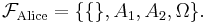$\textstyle \mathcal F_\text{Alice} = \{ \{\}, A_1, A_2, \Omega \}.$ Bob knows only the total number of heads. His partition $\textstyle \Omega = B_0 \uplus B_1 \uplus B_2 \uplus B_3 = \{TTT\} \uplus \{HTT, THT, TTH\} \uplus \{HHT, HTH, THH\} \uplus \{HHH\}$ contains 4 parts; accordingly, his σ-algebra $\textstyle \mathcal F_\text{Bob}$ contains $\textstyle 2^4 = 16$ events (just one of them: $\textstyle B_1 \uplus B_3 = \{HTT, THT, TTH, HHH\}$ ). 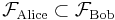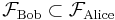The two σ-algebras are incomparable (neither $\textstyle \mathcal F_\text{Alice} \subset \mathcal F_\text{Bob}$ nor $\textstyle \mathcal F_\text{Bob} \subset \mathcal F_\text{Alice}$ ); both are sub-σ-algebras of $\textstyle 2^\Omega.$

Example 3

If 100 voters are to be drawn randomly from among all voters in California and asked whom they will vote for governor, then the set of all sequences of 100 Californian voters would be the sample space $\textstyle \Omega.$ (Assuming that sampling without replacement is used, only sequences of 100 different voters are allowed. Ordered sample is considered; otherwise 100-element sets of voters should be considered instead of sequences.)

The set of all sequences of 100 Californian voters in which at least 60 will vote for Schwarzenegger is identified with the event that at least 60 of the 100 chosen voters will so vote.

Alice knows only, whether this specific event occurs or not. Her incomplete information is described by the σ-algebra $\textstyle \mathcal F_\text{Alice}$ that contains: (1) the set of all sequences of 100 where at least 60 vote for Schwarzenegger; (2) the set of all sequences of 100 where fewer than 60 vote for Schwarzenegger (the complement of (1)); (3) the whole sample space Ω as above; and (4) the empty set.

Bob knows the number of voters who will vote for Schwarzenegger in the sample of 100. His incomplete information is described by the corresponding partition $\textstyle \Omega = B_0 \uplus B_1 \dots \uplus B_{100}$ (assuming that all these sets are nonempty, which depends on Californian voters...) and the σ-algebra $\textstyle \mathcal F_\text{Bob}$ of $\textstyle 2^{101}$ events. 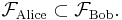$\textstyle \mathcal F_\text{Alice} \subset \mathcal F_\text{Bob}.$ The complete information is described by the much larger σ-algebra $\textstyle 2^\Omega$ of $\textstyle 2^{n(n-1)\dots(n-99)}$ events, where $\textstyle n$ is the number of all voters in California.

Non-atomic examples

Example 4

A number between $\textstyle 0$ and $\textstyle 1$ is chosen at random, uniformly. Here $\textstyle \Omega = [0,1],$ $\textstyle P$ is the Lebesgue measure on $\textstyle [0,1],$ and $\textstyle \mathcal F$ is the σ-algebra of all measurable subsets of $\textstyle [0,1].$ (The set $\textstyle (0,1)$ may be used equally well, since $\textstyle P ( \{0,1\} ) = 0.$ )

Intervals (or their finite unions) may be used as elementary sets.

Example 5

A fair coin is tossed endlessly. Here one can take $\textstyle \Omega = \{0,1\}^\infty,$ the set of all infinite sequences of numbers 0 and 1. Cylinder sets $\textstyle \{ (x_1,x_2,\dots) \in \Omega�: x_1=a_1, \dots, x_n=a_n \}$ (or their finite unions) may be used as elementary sets.

These two non-atomic examples are closely related: a sequence $\textstyle (x_1,x_2,\dots) \in \{0,1\}^\infty$ leads to the number $\textstyle \frac{x_1}{2^1} + \frac{x_2}{2^2} + \dots \in [0,1].$ This is not a one-to-one correspondence between $\textstyle \{0,1\}^\infty$ and $\textstyle [0,1]$ ; however, it is a isomorphism modulo zero, which allows for treating the two probability spaces as two forms of the same probability space. In fact, all non-pathologic non-atomic probability spaces are the same (in this sense), see standard probability space.

Related concepts

Probability distribution

Any probability distribution defines a probability measure.

Random variables

A random variable X is a measurable function from the sample space $\Omega$ ; to another measurable space called the state space.

If X is a real-valued random variable, then the notation ${\scriptstyle\Pr(X \geq 60)}$ is shorthand for ${\scriptstyle\Pr(\{ \omega \in \Omega \mid X(\omega) \geq 60 \})}$ , assuming that ${\scriptstyle X \geq 60}$ is an event.

Defining the events in terms of the sample space

If $\Omega$ is countable we almost always define $\mathcal F$ as the power set of $\Omega\,$ , i.e $\mathcal F=2^\Omega$ which is trivially a σ-algebra and the biggest one we can create using $\Omega\,$ . We can therefore omit $\mathcal{F}$ and just write $(\Omega,P)\,$ to define the probability space.

On the other hand, if $\Omega\,$ is uncountable and we use $\mathcal F=2^\Omega \,$ we get into trouble defining our probability measure $P\,$ because $\mathcal{F}$ is too 'huge', i.e. there will often be sets to which it will be impossible to assign a unique measure, giving rise to problems like the Banach–Tarski paradox. In this case, we have to use a smaller σ-algebra $\mathcal F$ (e.g. the Borel algebra of $\Omega\,$ , which is the smallest σ-algebra that makes all open sets measurable).

Conditional probability

Kolmogorov's definition of probability spaces gives rise to the natural concept of conditional probability. Every set $A$ with non-zero probability (that is, P(A) > 0 ) defines another probability measure

$P(B \vert A) = {P(B \cap A) \over P(A)}$

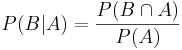
on the space. This is usually read as the "probability of B given A".

Independence

Two events, A and B are said to be independent if P(A∩B)=P(A)P(B).

Two random variables, X and Y, are said to be independent if any event defined in terms of X is independent of any event defined in terms of Y. Formally, they generate independent σ-algebras, where two σ-algebras G and H, which are subsets of F are said to be independent if any element of G is independent of any element of H.

The concept of independence is where probability theory departs from measure theory. In spite of defining independence as above the definition does not allow

further examination e.g. towards causation. Applications of the independence definition can lead type I, and II errors. Therefore, the definition leads to a blind alley.

It might be useful to apply Bayesian calculus for independent events, and to try to deduce equations as if independent formalism.

Mutual exclusivity

Two events, A and B are said to be mutually exclusive or disjoint if P(A∩B)=0. (This is weaker than A∩B=∅, which is the definition of disjoint for sets).

If A and B are disjoint events, then P(A∪B)=P(A)+P(B). This extends to a (finite or countably infinite) sequence of events. However, the probability of the union of an uncountable set of events is not the sum of their probabilities. For example, if Z is a normally distributed random variable, then P(Z=x) is 0 for any x, but P(Z is real)=1.

The event A∩B is referred to as A AND B, and the event A∪B as A OR B.

Bibliography

Pierre Simon de Laplace (1812) Analytical Theory of Probability

The first major treatise blending calculus with probability theory, originally in French: Théorie Analytique des Probabilités.

Andrei Nikolajevich Kolmogorov (1950) Foundations of the Theory of Probability

The modern measure-theoretic foundation of probability theory; the original German version (Grundbegriffe der Wahrscheinlichkeitrechnung) appeared in 1933.

Harold Jeffreys (1939) The Theory of Probability

An empiricist, Bayesian approach to the foundations of probability theory.

Edward Nelson (1987) Radically Elementary Probability Theory

Discrete foundations of probability theory, based on nonstandard analysis and internal set theory. downloadable. http://www.math.princeton.edu/~nelson/books.html

Patrick Billingsley: Probability and Measure, John Wiley and Sons, New York, Toronto, London, 1979.

Henk Tijms (2004) Understanding Probability

A lively introduction to probability theory for the beginner, Cambridge Univ. Press.

David Williams (1991) Probability with martingales

An undergraduate introduction to measure-theoretic probability, Cambridge Univ. Press.

Gut, Allan (2005). Probability: A Graduate Course. Springer. ISBN 0387228330.