Principal components analysis

Principal component analysis (PCA) is a vector space transform often used to reduce multidimensional data sets to lower dimensions for analysis. Depending on the field of application, it is also named the discrete Karhunen-Loève transform (KLT), the Hotelling transform or proper orthogonal decomposition (POD).

PCA was invented in 1901 by Karl Pearson^[1]. Now it is mostly used as a tool in exploratory data analysis and for making predictive models. PCA involves the calculation of the eigenvalue decomposition of a data covariance matrix or singular value decomposition of a data matrix, usually after mean centering the data for each attribute. The results of a PCA are usually discussed in terms of component scores and loadings (Shaw, 2003).

PCA is the simplest of the true eigenvector-based multivariate analyses. Often, its operation can be thought of as revealing the internal structure of the data in a way which best explains the variance in the data. If a multivariate dataset is visualised as a set of coordinates in a high-dimensional data space (1 axis per variable), PCA supplies the user with a lower-dimensional picture, a "shadow" of this object when viewed from its (in some sense) most informative viewpoint.

PCA is closely related to factor analysis; indeed, some statistical packages deliberately conflate the two techniques. True factor analysis makes different assumptions about the underlying structure and solves eigenvectors of a slightly different matrix.

1 Details
2 Discussion
3 Table of symbols and abbreviations
4 Properties and Limitations of PCA
5 Computing PCA using the Covariance Method
6 Derivation of PCA using the covariance method
7 Relation between PCA and K-means clustering
8 Correspondence analysis
9 Generalizations
- 9.1 Nonlinear generalizations
- 9.2 Higher order
10 Software/source code
11 Notes
12 References
13 See also
14 External links

Details

PCA is mathematically defined^[2] as an orthogonal linear transformation that transforms the data to a new coordinate system such that the greatest variance by any projection of the data comes to lie on the first coordinate (called the first principal component), the second greatest variance on the second coordinate, and so on. PCA is theoretically the optimum transform for a given data in least square terms.

PCA can be used for dimensionality reduction in a data set by retaining those characteristics of the data set that contribute most to its variance, by keeping lower-order principal components and ignoring higher-order ones. Such low-order components often contain the "most important" aspects of the data. However, depending on the application this may not always be the case.

For a data matrix, X^T, with zero empirical mean (the empirical mean of the distribution has been subtracted from the data set), where each row represents a different repetition of the experiment, and each column gives the results from a particular probe, the PCA transformation is given by:

$\mathbf{Y}^T=\mathbf{X}^T\mathbf{W}$

$= \mathbf{V}\mathbf{\Sigma}$

where V Σ W^T is the singular value decomposition (svd) of X^T.

PCA has the distinction of being the optimal linear transformation for keeping the subspace that has largest variance. This advantage, however, comes at the price of greater computational requirement if compared, for example, to the discrete cosine transform.

Discussion

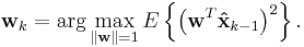
Though most derivations and implementations fail to identify the importance of mean subtraction, data centering is carried out because it is part of the solution towards finding a basis that minimizes the mean square error of approximating the data^[3]. Assuming zero empirical mean (the empirical mean of the distribution has been subtracted from the data set), the principal component w₁ of a data set x can be defined as:

$\mathbf{w}_1 = \arg\max_{\Vert \mathbf{w} \Vert = 1} \operatorname{var}\{ \mathbf{w}^T \mathbf{x} \} = \arg\max_{\Vert \mathbf{w} \Vert = 1} E\left\{ \left( \mathbf{w}^T \mathbf{x}\right)^2 \right\}$

(See arg max for the notation.) With the first $k - 1$ components, the $k$ ^th component can be found by subtracting the first $k - 1$ principal components from x:

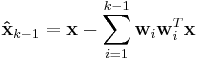
$\mathbf{\hat{x}}_{k - 1} = \mathbf{x} - \sum_{i = 1}^{k - 1} \mathbf{w}_i \mathbf{w}_i^T \mathbf{x}$

and by substituting this as the new data set to find a principal component in

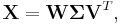
$\mathbf{w}_k = \arg\max_{\Vert \mathbf{w} \Vert = 1} E\left\{ \left( \mathbf{w}^T \mathbf{\hat{x}}_{k - 1} \right)^2 \right\}.$

The Karhunen-Loève transform is therefore equivalent to finding the singular value decomposition of the data matrix X,

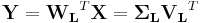
$\mathbf{X}=\mathbf{W}\mathbf{\Sigma}\mathbf{V}^T,$

and then obtaining the reduced-space data matrix Y by projecting X down into the reduced space defined by only the first L singular vectors, W_L:

$\mathbf{Y}=\mathbf{W_L}^T\mathbf{X} = \mathbf{\Sigma_L}\mathbf{V_L}^T$

The matrix W of singular vectors of X is equivalently the matrix W of eigenvectors of the matrix of observed covariances C = X X^T,

$\mathbf{X}\mathbf{X}^T = \mathbf{W}\mathbf{\Sigma}\mathbf{\Sigma}^T\mathbf{W}^T$

The eigenvectors with the largest eigenvalues correspond to the dimensions that have the strongest correlation in the data set (see Rayleigh quotient).

PCA is equivalent to empirical orthogonal functions (EOF).

An autoencoder neural network with a linear hidden layer is similar to PCA. Upon convergence, the weight vectors of the K neurons in the hidden layer will form a basis for the space spanned by the first K principal components. Unlike PCA, this technique will not necessarily produce orthogonal vectors.

PCA is a popular technique in pattern recognition. But it is not optimized for class separability^[4]. An alternative is the linear discriminant analysis, which does take this into account. PCA optimally minimizes reconstruction error under the L2 norm.

Table of symbols and abbreviations

Symbol	Meaning	Dimensions	Indices
$\mathbf{X} = \{ X[m,n] \}$	data matrix, consisting of the set of all data vectors, one vector per column	$M \times N$	$m = 1 \ldots M$ $n = 1 \ldots N$
$N \,$	the number of column vectors in the data set	$1 \times 1$	scalar
$M \,$	the number of elements in each column vector (dimension)	$1 \times 1$	scalar
$L \,$	the number of dimensions in the dimensionally reduced subspace, $1 \le L \le M$	$1 \times 1$	scalar
$\mathbf{u} = \{ u[m] \}$	vector of empirical means, one mean for each row m of the data matrix	$M \times 1$	$m = 1 \ldots M$
$\mathbf{s} = \{ s[m] \}$	vector of empirical standard deviations, one standard deviation for each row m of the data matrix	$M \times 1$	$m = 1 \ldots M$
$\mathbf{h} = \{ h[n] \}$	vector of all 1's	$1 \times N$	$n = 1 \ldots N$
$\mathbf{B} = \{ B[m,n] \}$	deviations from the mean of each row m of the data matrix	$M \times N$	$m = 1 \ldots M$ $n = 1 \ldots N$
$\mathbf{Z} = \{ Z[m,n] \}$	z-scores, computed using the mean and standard deviation for each row m of the data matrix	$M \times N$	$m = 1 \ldots M$ $n = 1 \ldots N$
$\mathbf{C} = \{ C[p,q] \}$	covariance matrix	$M \times M$	$p = 1 \ldots M$ $q = 1 \ldots M$
$\mathbf{R} = \{ R[p,q] \}$	correlation matrix	$M \times M$	$p = 1 \ldots M$ $q = 1 \ldots M$
$\mathbf{V} = \{ V[p,q] \}$	matrix consisting of the set of all eigenvectors of C, one eigenvector per column	$M \times M$	$p = 1 \ldots M$ $q = 1 \ldots M$
$\mathbf{D} = \{ D[p,q] \}$	diagonal matrix consisting of the set of all eigenvalues of C along its principal diagonal, and 0 for all other elements	$M \times M$	$p = 1 \ldots M$ $q = 1 \ldots M$
$\mathbf{W} = \{ W[p,q] \}$	matrix of basis vectors, one vector per column, where each basis vector is one of the eigenvectors of C, and where the vectors in W are a sub-set of those in V	$M \times L$	$p = 1 \ldots M$ $q = 1 \ldots L$
$\mathbf{Y} = \{ Y[m,n] \}$	matrix consisting of N column vectors, where each vector is the projection of the corresponding data vector from matrix X onto the basis vectors contained in the columns of matrix W.	$L \times N$	$m = 1 \ldots L$ $n = 1 \ldots N$

Properties and Limitations of PCA

PCA is theoretically the optimal linear scheme, in terms of least mean square error, for compressing a set of high dimensional vectors into a set of lower dimensional vectors and then reconstructing the original set. It is a non-parametric analysis and the answer is unique and independent of any hypothesis about data probability distribution. However, the latter two properties are regarded as weakness as well as strength, in that being non-parametric, no prior knowledge can be incorporated and that PCA compressions often incur loss of information.

The applicability of PCA is limited by the assumptions^[5] made in its derivation. These assumptions are:

Assumption on Linearity

We assumed the observed data set to be linear combinations of certain basis. Non-linear methods such as kernel PCA have been developed without assuming linearity.

Assumption on the statistical importance of mean and covariance

PCA uses the eigenvectors of the covariance matrix and it only finds the independent axes of the data under the Gaussian assumption. For non-Gaussian or multi-modal Gaussian data, PCA simply de-correlates the axes. When PCA is used for clustering, its main limitation is that it does not account for class separability since it makes no use of the class label of the feature vector. There is no guarantee that the directions of maximum variance will contain good features for discrimination.

Assumption that large variances have important dynamics

PCA simply performs a coordinate rotation that aligns the transformed axes with the directions of maximum variance. It is only when we believe that the observed data has a high signal-to-noise ratio that the principal components with larger variance correspond to interesting dynamics and lower ones correspond to noise.

Essentially, PCA involves only rotation and scaling. The above assumptions are made in order to simplify the algebraic computation on the data set. Some other methods have been developed without one or more of these assumptions; these are briefly described below.

Computing PCA using the Covariance Method

Following is a detailed description of PCA using the covariance method. The goal is to transform a given data set X of dimension M to an alternative data set Y of smaller dimension L. Equivalently, we are seeking to find the matrix Y, where Y is the Karhunen-Loeve transform (KLT) of matrix X:

$\mathbf{Y} = \mathbb{KLT} \{ \mathbf{X} \}$

Organize the data set

Suppose you have data comprising a set of observations of M variables, and you want to reduce the data so that each observation can be described with only L variables, L < M. Suppose further, that the data are arranged as a set of N data vectors $\mathbf{x}_1 \ldots \mathbf{x}_N$ with each $\mathbf{x}_n$ representing a single grouped observation of the M variables.

Write $\mathbf{x}_1 \ldots \mathbf{x}_N$ as column vectors, each of which has M rows.
Place the column vectors into a single matrix X of dimensions M × N.

Calculate the empirical mean

Find the empirical mean along each dimension m = 1...M.
Place the calculated mean values into an empirical mean vector u of dimensions M × 1.

$u[m] = {1 \over N} \sum_{n=1}^N X[m,n]$

Calculate the deviations from the mean

Mean subtraction is an integral part of the solution towards finding a principal component basis that minimizes the mean square error of approximating the data^[6]. Hence we proceed by centering the data as follows:

Subtract the empirical mean vector u from each column of the data matrix X.
Store mean-subtracted data in the M × N matrix B.

$\mathbf{B} = \mathbf{X} - \mathbf{u}\mathbf{h}$

where h is a 1 x N row vector of all 1's:

$h[n] = 1 \, \qquad \qquad \mathrm{for \ } n = 1 \ldots N$

Find the covariance matrix

Find the M × M empirical covariance matrix C from the outer product of matrix B with itself:

$\mathbf{C} = \mathbb{ E } \left[ \mathbf{B} \otimes \mathbf{B} \right] = \mathbb{ E } \left[ \mathbf{B} \cdot \mathbf{B}^{*} \right] = { 1 \over N } \mathbf{B} \cdot \mathbf{B}^{*}$

where

$\mathbb{E}$ is the expected value operator,

$\otimes$ is the outer product operator, and

$* \$ is the conjugate transpose operator. Note that if B consists entirely of real numbers, which is the case in many applications, the "conjugate transpose" is the same as the regular transpose.

Please note that the information in this section is indeed a bit fuzzy. See the covariance matrix sections on the discussion page for more information.

Find the eigenvectors and eigenvalues of the covariance matrix

Compute the matrix V of eigenvectors which diagonalizes the covariance matrix C:

$\mathbf{V}^{-1} \mathbf{C} \mathbf{V} = \mathbf{D}$

where D is the diagonal matrix of eigenvalues of C. This step will typically involve the use of a computer-based algorithm for computing eigenvectors and eigenvalues. These algorithms are readily available as sub-components of most matrix algebra systems, such as MATLAB^[7], Mathematica^[8], SciPy, or IDL(Interactive Data Language).

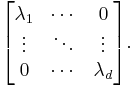
Matrix D will take the form of an M × M diagonal matrix, where

$D[p,q] = \lambda_m \qquad \mathrm{for} \qquad p = q = m$

is the mth eigenvalue of the covariance matrix C, and

$D[p,q] = 0 \qquad \mathrm{for} \qquad p \ne q.$

Matrix V, also of dimension M × M, contains M column vectors, each of length M, which represent the M eigenvectors of the covariance matrix C.
The eigenvalues and eigenvectors are ordered and paired. The mth eigenvalue corresponds to the mth eigenvector.

Rearrange the eigenvectors and eigenvalues

Sort the columns of the eigenvector matrix V and eigenvalue matrix D in order of decreasing eigenvalue.
Make sure to maintain the correct pairings between the columns in each matrix.

Compute the cumulative energy content for each eigenvector

The eigenvalues represent the distribution of the source data's energy among each of the eigenvectors, where the eigenvectors form a basis for the data. The cumulative energy content g for the mth eigenvector is the sum of the energy content across all of the eigenvectors from 1 through m:

$g[m] = \sum_{q=1}^m D[p,q] \qquad \mathrm{for} \qquad p = q \qquad \mathrm{and} \qquad m = 1...M$

Select a subset of the eigenvectors as basis vectors

Save the first L columns of V as the M × L matrix W:

$W[p,q] = V[p,q] \qquad \mathrm{for} \qquad p = 1...M \qquad q = 1...L$

where

$1 \leq L \leq M.$

Use the vector g as a guide in choosing an appropriate value for L. The goal is to choose as small a value of L as possible while achieving a reasonably high value of g on a percentage basis. For example, you may want to choose L so that the cumulative energy g is above a certain threshold, like 90 percent. In this case, choose the smallest value of L such that

$g[m=L] \ge 90%$

Convert the source data to z-scores

Create an M × 1 empirical standard deviation vector s from the square root of each element along the main diagonal of the covariance matrix C:

$\mathbf{s} = \{ s[m] \} = \sqrt{C[p,q]} \qquad \mathrm{for \ } p = q = m = 1 \ldots M$

Calculate the M × N z-score matrix:

$\mathbf{Z} = { \mathbf{B} \over \mathbf{s} \cdot \mathbf{h} }$ (divide element-by-element)

Note: While this step is useful for various applications as it normalizes the data set with respect to its variance, it is not integral part of PCA/KLT!

Project the z-scores of the data onto the new basis

The projected vectors are the columns of the matrix

$\mathbf{Y} = \mathbf{W}^* \cdot \mathbf{Z} = \mathbb{KLT} \{ \mathbf{X} \}.$

The columns of matrix Y represent the Karhunen-Loeve transforms (KLT) of the data vectors in the columns of matrix X.

Derivation of PCA using the covariance method

Let X be a d-dimensional random vector expressed as column vector. Without loss of generality, assume X has zero empirical mean. We want to find a $d \times d$ orthonormal transformation matrix P such that

$\mathbf{Y} = \mathbf{P}^\top \mathbf{X}$

with the constraint that

$\operatorname{cov}(\mathbf{Y})$ is a diagonal matrix and $\mathbf{P}^{-1} = \mathbf{P}^\top.$

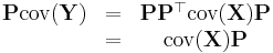
By substitution, and matrix algebra, we obtain:

$\begin{matrix} \operatorname{cov}(\mathbf{Y}) &=& \mathbb{E}[ \mathbf{Y} \mathbf{Y}^\top]\\ \ &=& \mathbb{E}[( \mathbf{P}^\top \mathbf{X} ) ( \mathbf{P}^\top \mathbf{X} )^\top]\\ \ &=& \mathbb{E}[(\mathbf{P}^\top \mathbf{X}) (\mathbf{X}^\top \mathbf{P})] \\ \ &=& \mathbf{P}^\top \mathbb{E}[\mathbf{X} \mathbf{X}^\top] \mathbf{P} \\ \ &=& \mathbf{P}^\top \operatorname{cov}(\mathbf{X}) \mathbf{P} \end{matrix}$

We now have:

$\begin{matrix} \mathbf{P}\operatorname{cov}(\mathbf{Y}) &=& \mathbf{P} \mathbf{P}^\top \operatorname{cov}(\mathbf{X}) \mathbf{P}\\ \ &=& \operatorname{cov}(\mathbf{X}) \mathbf{P}\\ \end{matrix}$

Rewrite P as d $d \times 1$ column vectors, so

$\mathbf{P} = [P_1, P_2, \ldots, P_d]$

and $\operatorname{cov}(\mathbf{Y})$ as:

$\begin{bmatrix} \lambda_1 & \cdots & 0 \\ \vdots & \ddots & \vdots \\ 0 & \cdots & \lambda_d \end{bmatrix}.$

Substituting into equation above, we obtain:

$[\lambda_1 P_1, \lambda_2 P_2, \ldots, \lambda_d P_d] = [\operatorname{cov}(X)P_1, \operatorname{cov}(X)P_2, \ldots, \operatorname{cov}(X)P_d].$

Notice that in 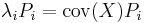$\lambda_i P_i = \operatorname{cov}(X)P_i$ , P_i is an eigenvector of X′s covariance matrix. Therefore, by finding the eigenvectors of X′s covariance matrix, we find a projection matrix P that satisfies the original constraints.

Relation between PCA and K-means clustering

It has been shown recently (2007) ^[9] ^[10] that the relaxed solution of K-means clustering, specified by the cluster indicators, is given by the PCA principal components, and the PCA subspace spanned by the principal directions is identical to the cluster centroid subspace specified by the between-class scatter matrix. Thus PCA automatically projects to the subspace where the global solution of K-means clustering lie, and thus facilitate K-means clustering to find near-optimal solutions.

Correspondence analysis

Correspondence analysis was developed by Jean-Paul Benzécri^[11] and is conceptually similar to PCA, but scales the data (which must be positive) so that rows and columns are treated equivalently. It is traditionally applied to contingency tables. Correspondence analysis decomposes the Chi-square statistic associated to this table into orthogonal factors^[12]. Because correspondence analysis is a descriptive technique, it can be applied to tables for which the Chi-square statistic is appropriate or not.

Generalizations

Nonlinear generalizations

Most of the modern methods for nonlinear dimensionality reduction find their theoretical and algorithmic roots in PCA or K-means. The original Pearson's idea was to take a straight line (or plane) which will be "the best fit" to a set of data points. Principal curves and manifolds give the natural geometric framework for PCA generalization and extend the geometric interpretation of PCA by explicitly constructing an embedded manifold for data approximation, and by encoding using standard geometric projection onto the manifold^[13]. See principal geodesic analysis.

Higher order

N-way principal component analysis may be performed with models like PARAFAC and Tucker decomposition.

Software/source code

"Spectramap" is software to create a biplot using principal components analysis, correspondence analysis or spectral map analysis.
Computer Vision Library
Multivariate Data Analysis Software
in Matlab, the function "wmspca" gives the principal component
in Octave, the free software equivalent to Matlab, the function princomp gives the principal component
in the open source statistical package R, the functions "princomp" and "prcomp" can be used for principal component analysis; prcomp uses singular value decomposition which generally gives better numerical accuracy.
"spm" is a generic package developed in R for multivariate projection methods that allows principal components analysis, correspondence analysis, and spectral map analysis
In XLMiner, the Principles Component tab can be used for principal component analysis.
SciLab
In IDL, the principal components can be calculated using the function pcomp.
Weka computes principal components (javadoc).

Notes

↑ Pearson, K. (1901). "On Lines and Planes of Closest Fit to Systems of Points in Space". Philosophical Magazine 2 (6): 559–572. http://stat.smmu.edu.cn/history/pearson1901.pdf.
↑ Jolliffe I.T. Principal Component Analysis, Series: Springer Series in Statistics, 2nd ed., Springer, NY, 2002, XXIX, 487 p. 28 illus. ISBN 978-0-387-95442-4
↑ A.A. Miranda, Y.-A. Le Borgne, and G. Bontempi. New Routes from Minimal Approximation Error to Principal Components, Volume 27, Number 3 / June, 2008, Neural Processing Letters, Springer
↑ Fukunaga, Keinosuke (1990). Introduction to Statistical Pattern Recognition. Elsevier. http://books.google.com/books?vid=ISBN0122698517.
↑ Jon Shlens, A Tutorial on Principal Component Analysis.
↑ A.A. Miranda, Y.-A. Le Borgne, and G. Bontempi. New Routes from Minimal Approximation Error to Principal Components, Volume 27, Number 3 / June, 2008, Neural Processing Letters, Springer
↑ eig function Matlab documentation
↑ Eigenvalues function Mathematica documentation
↑ H. Zha, C. Ding, M. Gu, X. He and H.D. Simon. "Spectral Relaxation for K-means Clustering", http://ranger.uta.edu/~chqding/papers/Zha-Kmeans.pdf, Neural Information Processing Systems vol.14 (NIPS 2001). pp. 1057-1064, Vancouver, Canada. Dec. 2001.
↑ C. Ding and X. He. "K-means Clustering via Principal Component Analysis". Proc. of Int'l Conf. Machine Learning (ICML 2004), pp 225-232. July 2004. http://ranger.uta.edu/~chqding/papers/KmeansPCA1.pdf
↑ Benzécri, J.-P. (1973). L'Analyse des Données. Volume II. L'Analyse des Correspondences. Paris, France: Dunod.
↑ Greenacre, Michael (1983). Theory and Applications of Correspondence Analysis. London: Academic Press. ISBN 0-12-299050-1.
↑ A. Gorban, B. Kegl, D. Wunsch, A. Zinovyev (Eds.), Principal Manifolds for Data Visualisation and Dimension Reduction, LNCSE 58, Springer, Berlin - Heidelberg - New York, 2007. ISBN 978-3-540-73749-0

References

R. Kramer, Chemometric Techniques for Quantitative Analysis, (1998) Marcel-Dekker, ISBN: 0-8247-0198-4.
Shaw PJA, Multivariate statistics for the Environmental Sciences, (2003) Hodder-Arnold.
Patra sk et al., J- Photochemistry & Photobiology A:Chemistry, (1999) 122:23-31

External links

Data compression methods

Lossless

Theory	Entropy · Complexity · Redundancy

Entropy encoding	Huffman · Adaptive Huffman · Arithmetic (Shannon-Fano · Range) · Golomb · Exp-Golomb · Universal (Elias · Fibonacci)

Dictionary	RLE · DEFLATE · LZ Family (LZ77/78 · LZSS · LZW · LZWL · LZO · LZMA · LZX · LZJB · LZT)

Others	CTW · BWT · PPM · DMC

Audio

Theory	Convolution · Sampling · Nyquist–Shannon theorem

Audio codec parts	LPC (LAR · LSP) · WLPC · CELP · ACELP · A-law · μ-law · MDCT · Fourier transform · Psychoacoustic model

Others	Dynamic range compression · Speech compression · Sub-band coding

Image

Terms	Color space · Pixel · Chroma subsampling · Compression artifact

Methods	RLE · Fractal · Wavelet · EZW · SPIHT · DCT · KLT

Others	Bit rate · Test images · PSNR quality measure · Quantization

Video

Terms	Video Characteristics · Frame · Frame types · Video quality

Video codec parts	Motion compensation · DCT · Quantization

Others	Video codecs · Rate distortion theory (CBR · ABR · VBR)

Timeline of information theory, data compression, and error-correcting codes

See Compression Formats and Standards for formats and Compression Software Implementations for codecs