Permutation

In several fields of mathematics the term permutation is used with different but closely related meanings. They all relate to the notion of mapping the elements of a set to other elements of the same set, i.e., exchanging (or "permuting") elements of a set.

Definitions

The general concept of permutation can be defined more formally in different contexts:

In combinatorics

In combinatorics, a permutation is usually understood to be a sequence containing each element from a finite set once, and only once. The concept of sequence is distinct from that of a set, in that the elements of a sequence appear in some order: the sequence has a first element (unless it is empty), a second element (unless its length is less than 2), and so on. In contrast, the elements in a set have no order; {1, 2, 3} and {3, 2, 1} are different ways to denote the same set.

However, there is also a traditional more general meaning of the term "permutation" used in combinatorics. In this more general sense, permutations are those sequences in which, as before, each element occurs at most once, but not all elements of the given set need to be used.

For a related notion in which the ordering of the selected elements form a set, for which the ordering is irrelevant, see Combination.

In group theory

In group theory and related areas, the elements of a permutation need not be arranged in a linear order, or indeed in any order at all. Under this refined definition, a permutation is a bijection from a finite set onto itself. This allows for the definition of groups of permutations; see Permutation group.

Counting permutations

In this section only, the traditional definition from combinatorics is used: a permutation is an ordered sequence of elements selected from a given finite set, without repetitions, and not necessarily using all elements of the given set. For example, given the set of letters {C, E, G, I, N, R}, some permutations are ICE, RING, RICE, NICER, REIGN and CRINGE, but also RNCGI – the sequence need not spell out an existing word. ENGINE, on the other hand, is not a permutation, because it uses the elements E and N twice.

If n denotes the size of the set – the number of elements available for selection – and only permutations are considered that use all n elements, then the total number of possible permutations is equal to n!, where "!" is the factorial operator. This can be shown informally as follows. In constructing a permutation, there are n possible choices for the first element of the sequence. Once it has been chosen, n − 1 elements are left, so for the second element there are only n − 1 possible choices. For the first two elements together, that gives us

n × (n − 1) possible permutations.

For selecting the third element, there are then n − 2 elements left, giving, for the first three elements together,

n × (n − 1) × (n − 2) possible permutations.

Continuing in this way until there are only 2 elements left, there are 2 choices, giving for the number of possible permutations consisting of n − 1 elements:

n × (n − 1) × (n − 2) × ... × 2.

The last choice is now forced, as there is exactly one element left. In a formula, this is the number

n × (n − 1) × (n − 2) × ... × 2 × 1

(which is the same as before because the factor 1 does not make a difference). This number is, by definition, the same as n!.

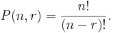
In general the number of permutations is denoted by P(n, r), _nP_r, or sometimes $P_r^n$ , where:

n is the number of elements available for selection, and
r is the number of elements to be selected (0 ≤ r ≤ n).

For the case where r = n it has just been shown that P(n, r) = n!. The general case is given by the formula:

$P(n, r) = \frac{n!}{(n-r)!}.$

As before, this can be shown informally by considering the construction of an arbitrary permutation, but this time stopping when the length r has been reached. The construction proceeds initially as above, but stops at length r. The number of possible permutations that has then been reached is:

P(n, r) = n × (n − 1) × (n − 2) × ... × (n − r + 1).

So:

n! = n × (n − 1) × (n − 2) × ... × 2 × 1

= n × (n − 1) × (n − 2) × ... × (n − r + 1) × (n − r) × ... × 2 × 1

= P(n, r) × (n − r) × ... × 2 × 1

= P(n, r) × (n − r)!.

But if n! = P(n, r) × (n − r)!, then P(n, r) = n! / (n − r)!.

For example, if there is a total of 10 elements and we are selecting a sequence of three elements from this set, then the first selection is one from 10 elements, the next one from the remaining 9, and finally from the remaining 8, giving 10 × 9 × 8 = 720. In this case, n = 10 and r = 3. Using the formula to calculate P(10,3),

$P(10,3) = \frac{10!}{(10-3)!} = \frac{10!}{7!} = \frac{7!\times 8 \times 9 \times 10}{7!} = 8 \times 9 \times 10 = 720.$

In the special case where n = r the formula above simplifies to:

$P(n,r) = \frac{n!}{0!} = \frac{n!}{1} = n!.$

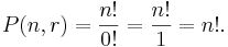
The reason why 0! = 1 is that 0! is an empty product, which always equals 1.

In the example given in the header of this article, with 6 integers {1..6}, this would be: P(6,6) = 6! / (6−6)! = (1×2×3×4×5×6) / 0! = 720 / 1 = 720.

Since it may be impractical to calculate $n!$ if the value of n is very large, a more efficient algorithm is to calculate:

P(n, r) = n × (n − 1) × (n − 2) × ... × (n − r + 1).

Other, older notations include ⁿP_r, P_n,r, or _nP_r. A common modern notation is (n)_r which is called a falling factorial. However, the same notation is used for the rising factorial (also called Pochhammer symbol)

n(n + 1)(n + 2)⋯(n + r − 1)r.

With the rising factorial notation, the number of permutations is (n − r + 1)_r.

Permutations in group theory

As explained in a previous section, in group theory the term permutation (of a set) is reserved for a bijective map (bijection) from a finite set onto itself. The earlier example, of making permutations out of numbers 1 to 10, would be translated as a map from the set {1, …, 10} to itself.

Notation

There are two main notations for such permutations. In relation notation, one can just arrange the "natural" ordering of the elements being permuted on a row, and the new ordering on another row (first example below):

$\begin{pmatrix} 1 & 2 & 3 & 4 & 5 \\ 2 & 5 & 4 & 3 & 1\end{pmatrix} = (2,5,4,3,1) = \begin{pmatrix}1 & 2 & 5 \end{pmatrix} \begin{pmatrix}3 & 4 \end{pmatrix} = \begin{pmatrix}3 & 4 \end{pmatrix} \begin{pmatrix}1 & 2 & 5 \end{pmatrix}= \begin{pmatrix}3 & 4 \end{pmatrix} \begin{pmatrix}5 & 1 & 2 \end{pmatrix}$

stands for the permutation s of the set {1,2,3,4,5} defined by s(1)=2, s(2)=5, s(3)=4, s(4)=3, s(5)=1.

If we have a finite set E of n elements, it is by definition in bijection with the set {1,…,n}, where this bijection f corresponds just to numbering the elements. Once they are numbered, we can identify the permutations of the set E with permutations of the set {1,…,n}. (In more mathematical terms, the function that maps a permutation s of E to the permutation f o s o f⁻¹ of {1,…,n} is a morphism from the symmetric group of E into that of {1,…,n}, see below.)

Alternatively, we can write the permutation in terms of how the elements change when the permutation is successively applied. This is referred to as the permutation's decomposition in a product of disjoint cycles using cycle notation (last three examples above). It works as follows: starting from one element x, we write the sequence (x s(x) s²(x) …) until we get back the starting element (at which point we close the parenthesis without writing the starting element for a second time). This is called the cycle associated to x's orbit following s. Then we take an element we did not write yet and do the same thing, until we have considered all elements. In the above example, we get: s = (1 2 5) (3 4).

Each cycle (x₁ x₂ … x_L) stands for the permutation that maps x_i on x_i+1 (i=1…L−1) and x_L on x₁, and leaves all other elements invariant. L is called the length of the cycle. Since these cycles have by construction disjoint supports (i.e. they act non-trivially on disjoint subsets of E), they do commute (for example, (1 2 5) (3 4) = (3 4)(1 2 5)). The order of the cycles in the (composition) product does not matter, while the order of the elements in each cycles does matter (up to cyclic change; see also cycles and fixed points). The canonical way of representing such cycles is to start by the smallest element of each cycle.

A 1-cycle (cycle of length 1) simply fixes the element contained in it, so it is often not written explicitly. Some authors define a cycle to exclude cycles of length 1.

Cycles of length two are called transpositions; such permutations merely exchange the place of two elements. (Conversely, a matrix transposition is itself an important example of a permutation.)

Product and inverse of permutations

Main article: Symmetric group

One can define the product of two permutations as follows. If we have two permutations, P and Q, the action of first performing P and then Q will be the same as performing some single permutation R. The product of P and Q is then defined to be that permutation R. Viewing permutations as bijections, the product of two permutations is thus the same as their composition as functions. There is no universally agreed notation for the product operation between permutations, and depending on the author a formula like PQ may mean either P ∘ Q or Q ∘ P. Since function composition is associative, so is the product operation on permutations: (P ∘ Q) ∘ R = P ∘ (Q ∘ R).

Likewise, since bijections have inverses, so do permutations, and both P ∘ P⁻¹ and P⁻¹ ∘ P are the "identity permutation" (see below) that leaves all positions unchanged. Thus, it can be seen that permutations form a group.

As for any group, there is a group isomorphism on permutation groups, obtained by assigning to each permutation its inverse, and this isomorphism is an involution, giving a dual view on any abstract result. Since (P ∘ Q)⁻¹ = Q⁻¹ ∘ P⁻¹, from an abstract point of view it is immaterial whether PQ represents "P before Q" or "P after Q". For concrete permutations, the distinction is, of course, quite material.

Special permutations

If we think of a permutation that "changes" the position of the first element to the first element, the second to the second, and so on, we really have not changed the positions of the elements at all. Because of its action, we describe it as the identity permutation because it acts as an identity function. Conversely, a permutation which changes the position of all elements (no element is mapped to itself) is called a derangement.

If one has some permutation, called P, one may describe a permutation, written P⁻¹, which undoes the action of applying P. In essence, performing P then P⁻¹ is equivalent to performing the identity permutation. One always has such a permutation since a permutation is a bijective map. Such a permutation is called the inverse permutation. It is computed by exchanging each number and the number of the place which it occupies.

An even permutation is a permutation which can be expressed as the product of an even number of transpositions, and the identity permutation is an even permutation as it equals (1 2)(1 2). An odd permutation is a permutation which can be expressed as the product of an odd number of transpositions. It can be shown that every permutation is either odd or even and can't be both.

One theorem regarding the inverse permutation is the effect of a conjugation of a permutation by a permutation in a permutation group. If we have a permutation Q=(i₁ i₂ … i_n) and a permutation P, then PQP⁻¹ = (P(i₁) P(i₂) … P(i_n)).

We can also represent a permutation in matrix form; the resulting matrix is known as a permutation matrix.

Properties of permutations

Ascents, descents and runs

An ascent in a permutation is any position i where the following value is bigger than the current one. That is, if $p=p_1p_2\dots p_n$ is a permutation, then any position i with $p_i< p_{i+1}$ is called an ascent.

For example, the permutation 3452167 has the ascends 1,2,5,6.

Similarly, a descent is a position i with $p_i> p_{i+1}$ .

The number of permutations with a given number of ascents or descents is equal to the Eulerian Number $A(n,k)$ , where n is the number of elements of the permutation and k is the the given number of ascents or descents.^[1]

For example, the permutation 3452167 has the ascending runs 345,2,167.

A ascending run of a permutation is a subsequence of the permutation in which the values raise from position to position. If a permutation has $k-1$ descents, then it must be the union of k ascending runs. Hence, the number of permutations with k ascending runs is the same as the the number of permutations with $k-1$ descents.^[2]

Inversions

An inversion, is a pair of entries of a permutation which appear in ascending order, even though the entry that appears first is greater than the entry that appears second.^[3]

For example, the permutation 23154 has three inversions: $(2,1), (3,1),(5,4)$ .

The number of permutations with k inversions is expressed by Mahonian numbers^[4]

Permutations in computing

Some of the older textbooks look at permutations as assignments, as mentioned above. In computer science terms, these are assignment operations, with values

1, 2, …, n

assigned to variables

x₁, x₂, …, x_n.

Each value should be assigned only once.

The assignment/substitution difference is then illustrative of one way in which functional programming and imperative programming differ — pure functional programming has no assignment mechanism. The mathematics convention is nowadays that permutations are just functions and the operation on them is function composition; functional programmers follow this. In the assignment language a substitution is an instruction to switch round the values assigned, simultaneously; a well-known problem.

Numbering permutations

Factoradic numbers can be used to assign unique numbers to permutations, such that given a factoradic of k one can quickly find the corresponding permutation.

Algorithms to generate permutations

Unordered generation

For every number k, with 0 ≤ k < n!, the following algorithm generates a unique permutation of the initial sequence s_j, j=1…n:

 function permutation(k, s) {
     for j= 2 to length(s) {
        k:= k/ (j-1);        // integer division cuts off the remainder
        swap s[(k mod j)+ 1] with s[j]; //note that our array is indexed starting at 1
     }
     return s;
 }

The first line in the for loop is constructing the Factorial base representation of k -- the important thing here is that for each k, it generates a unique corresponding sequence of n integers where the first number is in {0,1}, the second is in {0,1,2}, etc. Thus what the second line is doing is , at each step, swapping the jth element with one of the elements that are currently before it. If we consider the swaps in reverse order, we see that it implements a backwards Selection sort, first putting the nth element in the correct place, then the n-1st, etc. Since there is exactly one way to selection sort a permutation, this algorithm generates a unique permutation for each choice of k.

The Fisher-Yates shuffle is based on the same principle as this algorithm.

Lexicographical order generation

For every number k, with 0 ≤ k < n!, the following algorithm generates the corresponding lexicographical permutation of the initial sequence s_j, j= 1…n:

 function permutation(k, s) {
     var int n:= length(s); factorial:= 1;
     for j= 2 to n- 1 {             // compute (n- 1)!
         factorial:= factorial* j;
     }
     for j= 1 to n- 1 {
         tempj:= (k/ factorial) mod (n+ 1- j);
         temps:= s[j+ tempj]
         for i= j+ tempj to j+ 1 step -1 {
             s[i]:= s[i- 1];      // shift the chain right
         }
         s[j]:= temps;
         factorial:= factorial/ (n- j);
     }
     return s;
 }

Notation

k / j denotes integer division of k by j, i.e. the integral quotient without any remainder, and
k mod j is the remainder following integer division of k by j.
s[n] denotes the nth element of sequence s.

Software and hardware implementations

Calculator functions

Most calculators have a built-in function for calculating the number of permutations, called nPr or PERM on many. The permutations function is often only available through several layers of menus; how to access the function is usually indicated in the documentation for calculators that support it.

Spreadsheet functions

Most spreadsheet software also provides a built-in function for calculating the number of permutations, called PERMUT in many popular spreadsheets. Apple's Numbers software notably does not currently include such a function.^[5]

Notes

↑ Combinatorics of Permutations, ISBN 1584884347, M. Bona, 2004, p. 3
↑ Combinatorics of Permutations, ISBN 1584884347, M. Bona, 2004, p. 4f
↑ Combinatorics of Permutations, ISBN 1584884347, M. Bona, 2004, p. 43
↑ Combinatorics of Permutations, ISBN 1584884347, M. Bona, 2004, p. 43ff
↑ Curmi, Jamie (2007-08-26). "Summary of Functions in Excel and Numbers" (PDF). Retrieved on 2007-10-19.

References

Miklos Bona. "Combinatorics of Permutations", Chapman Hall-CRC, 2004. ISBN 1-58488-434-7.
Donald Knuth. The Art of Computer Programming, Volume 4: Generating All Tuples and Permutations, Fascicle 2, first printing. Addison-Wesley, 2005. ISBN 0-201-85393-0.
Donald Knuth. The Art of Computer Programming, Volume 3: Sorting and Searching, Second Edition. Addison-Wesley, 1998. ISBN 0-201-89685-0. Section 5.1: Combinatorial Properties of Permutations, pp.11–72.

Permutation

Contents

Definitions

In combinatorics

In group theory

Counting permutations

Permutations in group theory

Notation

Product and inverse of permutations

Special permutations

Properties of permutations

Ascents, descents and runs

Inversions

Permutations in computing

Numbering permutations

Algorithms to generate permutations

Unordered generation

Lexicographical order generation

Software and hardware implementations

Calculator functions

Spreadsheet functions

See also

Notes

References

External links