Partial derivative

In mathematics, a partial derivative of a function of several variables is its derivative with respect to one of those variables with the others held constant (as opposed to the total derivative, in which all variables are allowed to vary). Partial derivatives are useful in vector calculus and differential geometry.

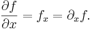
The partial derivative of a function f with respect to the variable x is written as f_x, ∂_xf, or ∂f/∂x. The partial-derivative symbol ∂ is a rounded letter, distinguished from the straight d of total-derivative notation. The notation was introduced by Adrien-Marie Legendre and gained general acceptance after its reintroduction by Carl Gustav Jacob Jacobi.

1 Introduction
2 Definition
3 Examples
4 Notation
5 Formal definition and properties
6 See also
7 References

Introduction

Suppose that ƒ is a function of more than one variable. For instance,

$f(x, y) = x^2 + xy + y^2.\,$

A graph of z = x² + xy + y². We want to find the partial derivative at (1, 1, 3) that leaves y constant; the corresponding tangent line is parallel to the x-axis.

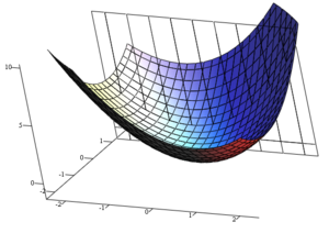
It is difficult to describe the derivative of such a function, as there are an infinite number of tangent lines to every point on this surface. Partial differentiation is the act of choosing one of these lines and finding its slope. Usually, the lines of most interest are those that are parallel to the x-axis, and those that are parallel to the y-axis.

This is a slice of the graph at the right at y = 1.

A good way to find these parallel lines is to treat the other variable as a constant. For example, to find the tangent line of the above function at (1, 1, 3) that is parallel to the x-axis, we treat y as a constant one. The graph and this plane are shown on the right. On the left, we see the way the function looks on the plane y = 1. By finding the tangent line on this graph, we discover that the slope of the tangent line of ƒ at (1, 1, 3) that is parallel to the x axis is three. We write this in notation as

$\frac{\part z}{\part x} = 3$

at the point (1, 1, 3),

or as "The partial derivative of z with respect to x at (1, 1, 3) is 3."

Definition

The function f can be reinterpreted as a family of functions of one variable indexed by the other variables:

$f(x,y) = f_x(y) = \,\! x^2 + xy + y^2.\,$

In other words, every value of x defines a function, denoted f_x, which is a function of one real number.^[1] That is,

$f_x(y) = x^2 + xy + y^2.\,$

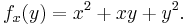
Once a value of x is chosen, say a, then f(x,y) determines a function f_a which sends y to a² + ay + y²:

$f_a(y) = a^2 + ay + y^2. \,$

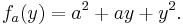
In this expression, a is a constant, not a variable, so f_a is a function of only one real variable, that being y. Consequently the definition of the derivative for a function of one variable applies:

$f_a'(y) = a + 2y. \,$

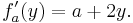
The above procedure can be performed for any choice of a. Assembling the derivatives together into a function gives a function which describes the variation of f in the y direction:

$\frac{\part f}{\part y}(x,y) = x + 2y.\,$

This is the partial derivative of f with respect to y. Here ∂ is a rounded d called the partial derivative symbol. To distinguish it from the letter d, ∂ is sometimes pronounced "der", "del", "dah", or "partial" instead of "dee".

In general, the partial derivative of a function f(x₁,...,x_n) in the direction x_i at the point (a₁,...,a_n) is defined to be:

$\frac{\part f}{\part x_i}(a_1,\ldots,a_n) = \lim_{h \to 0}\frac{f(a_1,\ldots,a_i+h,\ldots,a_n) - f(a_1,\ldots,a_n)}{h}.$

In the above difference quotient, all the variables except x_i are held fixed. That choice of fixed values determines a function of one variable $f_{a_1,\ldots,a_{i-1},a_{i+1},\ldots,a_n}(x_i) = f(a_1,\ldots,a_{i-1},x_i,a_{i+1},\ldots,a_n)$ , and by definition,

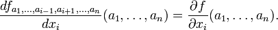
$\frac{df_{a_1,\ldots,a_{i-1},a_{i+1},\ldots,a_n}}{dx_i}(a_1,\ldots,a_n) = \frac{\part f}{\part x_i}(a_1,\ldots,a_n).$

In other words, the different choices of a index a family of one-variable functions just as in the example above. This expression also shows that the computation of partial derivatives reduces to the computation of one-variable derivatives.

An important example of a function of several variables is the case of a scalar-valued function f(x₁,...x_n) on a domain in Euclidean space Rⁿ (e.g., on R² or R³). In this case f has a partial derivative ∂f/∂x_j with respect to each variable x_j. At the point a, these partial derivatives define the vector

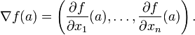
$\nabla f(a) = \left(\frac{\partial f}{\partial x_1}(a), \ldots, \frac{\partial f}{\partial x_n}(a)\right).$

This vector is called the gradient of f at a. If f is differentiable at every point in some domain, then the gradient is a vector-valued function ∇f which takes the point a to the vector ∇f(a). Consequently the gradient determines a vector field.

Examples

The volume of a cone depends on height and radius

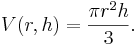
Consider the volume V of a cone; it depends on the cone's height h and its radius r according to the formula

$V(r, h) = \frac{\pi r^2 h}{3}.$

The partial derivative of V with respect to r is

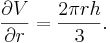
$\frac{ \partial V}{\partial r} = \frac{ 2 \pi r h}{3}.$

It describes the rate with which a cone's volume changes if its radius is varied and its height is kept constant. The partial derivative with respect to h is

$\frac{ \partial V}{\partial h} = \frac{\pi r^2}{3}$

and represents the rate with which the volume changes if its height is varied and its radius is kept constant.

Now consider by contrast the total derivative of V with respect to r and h. They are, respectively

$\frac{\operatorname dV}{\operatorname dr} = \overbrace{\frac{2 \pi r h}{3}}^\frac{ \partial V}{\partial r} + \overbrace{\frac{\pi r^2}{3}}^\frac{ \partial V}{\partial h}\frac{\partial h}{\partial r}$

and

$\frac{\operatorname dV}{\operatorname dh} = \overbrace{\frac{\pi r^2}{3}}^\frac{ \partial V}{\partial h} + \overbrace{\frac{2 \pi r h}{3}}^\frac{ \partial V}{\partial r}\frac{\partial r}{\partial h}$

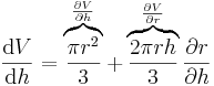
We see that the difference between the total and partial derivative is the elimination of indirect dependencies between variables in the latter.

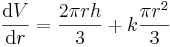
Now suppose that, for some reason, the cone's proportions have to stay the same, and the height and radius are in a fixed ratio k:

$k = \frac{h}{r} = \frac{\partial h}{\partial r}$

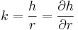
This gives the total derivative:

$\frac{\operatorname dV}{\operatorname dr} = \frac{2 \pi r h}{3} + k\frac{\pi r^2}{3}$

Equations involving an unknown function's partial derivatives are called partial differential equations and are common in physics, engineering, and other sciences and applied disciplines.

Notation

For the following examples, let f be a function in x, y and z.

First-order partial derivatives:

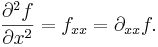
$\frac{ \partial f}{ \partial x} = f_x = \partial_x f.$

Second-order partial derivatives:

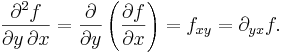
$\frac{ \partial^2 f}{ \partial x^2} = f_{xx} = \partial_{xx} f.$

Second-order mixed derivatives:

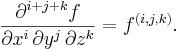
$\frac{\partial^2 f}{\partial y \, \partial x} = \frac{\partial}{\partial y} \left( \frac{\partial f}{\partial x} \right) = f_{xy} = \partial_{yx} f.$

Higher-order partial and mixed derivatives:

$\frac{ \partial^{i+j+k} f}{ \partial x^i\, \partial y^j\, \partial z^k } = f^{(i, j, k)}.$

When dealing with functions of multiple variables, some of these variables may be related to each other, and it may be necessary to specify explicitly which variables are being held constant. In fields such as statistical mechanics, the partial derivative of f with respect to x, holding y and z constant, is often expressed as

$\left( \frac{\partial f}{\partial x} \right)_{y,z}.$

Formal definition and properties

Like ordinary derivatives, the partial derivative is defined as a limit. Let U be an open subset of Rⁿ and f : U → R a function. We define the partial derivative of f at the point a = (a₁, ..., a_n) ∈ U with respect to the i-th variable x_i as

$\frac{ \partial }{\partial x_i }f(\mathbf{a}) = \lim_{h \rightarrow 0}{ f(a_1, \dots , a_{i-1}, a_i+h, a_{i+1}, \dots ,a_n) - f(a_1, \dots ,a_n) \over h }$

Even if all partial derivatives ∂f/∂x_i(a) exist at a given point a, the function need not be continuous there. However, if all partial derivatives exist in a neighborhood of a and are continuous there, then f is totally differentiable in that neighborhood and the total derivative is continuous. In this case, we say that f is a C¹ function. We can use this fact to generalize for vector valued functions (f : U → R'^m) by carefully using a componentwise argument.

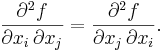
The partial derivative $\frac{\partial f}{\partial x}$ can be seen as another function defined on U and can again be partially differentiated. If all mixed second order partial derivatives are continuous at a point (or on a set), we call f a C² function at that point (or on that set); in this case, the partial derivatives can be exchanged by Clairaut's theorem:

$\frac{\partial^2f}{\partial x_i\, \partial x_j} = \frac{\partial^2f} {\partial x_j\, \partial x_i}.$

References

↑ This can also be expressed as the adjointness between the product space and function space constructions.