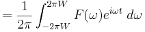
Nyquist–Shannon sampling theorem

The Nyquist–Shannon sampling theorem is a fundamental result in the field of information theory, in particular telecommunications and signal processing. Sampling is the process of converting a signal (for example, a function of continuous time or space) into a numeric sequence (a function of discrete time or space). The theorem states:[1]
If a function x(t) contains no frequencies higher than B cps, it is completely determined by giving its ordinates at a series of points spaced 1/(2B) seconds apart.
In essence the theorem shows that an analog signal that has been sampled can be perfectly reconstructed from the samples if the sampling rate exceeds 2B samples per second, where B is the highest frequency in the original signal. If a signal contains a component at exactly B hertz, then samples spaced at exactly 1/(2B) seconds do not completely determine the signal, Shannon's statement notwithstanding.
More recent statements of the theorem are sometimes careful to exclude the equality condition; that is, the condition is if x(t) contains no frequencies higher than or equal to B; this condition is equivalent to Shannon's except when the function includes a steady sinusoidal component at exactly frequency B.
The assumptions necessary to prove the theorem form a mathematical model that is only an idealization of any real-world situation. The conclusion that perfect reconstruction is possible is mathematically correct for the model but only an approximation for actual signals and actual sampling techniques.
The theorem also leads to a formula for reconstruction of the original signal.
Introduction
A signal or function is bandlimited if it contains no energy at frequencies higher than some bandlimit or bandwidth B. A signal that is bandlimited is constrained in how rapidly it changes in time, and therefore how much detail it can convey in an interval of time. The sampling theorem asserts that the uniformly spaced discrete samples are a complete representation of the signal if this bandwidth is less than half the sampling rate.
To formalize these concepts, let  represent a continuous-time signal and
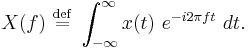
  be the continuous Fourier transform of that signal (which exists if is square-integrable):
The signal is bandlimited to a one-sided baseband bandwidth, B, if:
 for all
or, equivalently, the support of X supp(X)⊆[-B,B]. Then the sufficient condition for exact reconstructability from samples at a uniform sampling rate  (in samples per unit time) is:

or equivalently:

 is called the Nyquist rate and is a property of the bandlimited signal, while
  is called the Nyquist frequency and is a property of this sampling system.
The time interval between successive samples is referred to as the sampling interval:

and the samples of are denoted by:
 (integers).
The sampling theorem leads to a procedure for reconstructing the original  from the samples and states sufficient conditions for such a reconstruction to be exact.
The sampling process
The theorem describes two processes in signal processing: a sampling process, in which a continuous time signal is converted to a discrete time signal, and a reconstruction process, in which the original continuous signal is recovered from the discrete time signal.
The continuous signal varies over time (or space in a digitized image, or another independent variable in some other application) and the sampling process is performed by measuring the continuous signal's value every T units of time (or space), which is called the sampling interval. In practice, for signals that are a function of time, the sampling interval is typically quite small, on the order of milliseconds, microseconds, or less. This results in a sequence of numbers, called samples, to represent the original signal. Each sample value is associated with the instant in time when it was measured. The reciprocal of the sampling interval (1/T) is the sampling frequency denoted fs, which is measured in samples per unit of time. If T is expressed in seconds, then fs is expressed in Hz.
Reconstruction of the original signal is an interpolation process that mathematically defines a continuous-time signal x(t) from the discrete samples x[n] and at times in between the sample instants nT.

- The procedure: Each sample value is multiplied by the sinc function scaled so that the zero-crossings of the sinc function occur at the sampling instants and that the sinc function's central point is shifted to the time of that sample, nT. All of these shifted and scaled functions are then added together to recover the original signal. The scaled and time-shifted sinc functions are continuous making the sum of these also continuous, so the result of this operation is a continuous signal. This procedure is represented by the Whittaker–Shannon interpolation formula.
- The condition: The signal obtained from this reconstruction process can have no frequencies higher than one-half the sampling frequency. According to the theorem, the reconstructed signal will match the original signal provided that the original signal contains no frequencies at or above this limit. This condition is called the Nyquist criterion, or sometimes the Raabe condition.
If the original signal contains a frequency component equal to one-half the sampling rate, the condition is not satisfied. The resulting reconstructed signal may have a component at that frequency, but the amplitude and phase of that component generally will not match the original component.
This reconstruction or interpolation using sinc functions is not the only interpolation scheme. Indeed, it is impossible in practice because it requires summing an infinite number of terms. However, it is the interpolation method that in theory exactly reconstructs any given bandlimited x(t) with any bandlimit B < 1/2T); any other method that does so is formally equivalent to it.
Practical considerations
A few consequences can be drawn from the theorem:
- If the highest frequency B in the original signal is known, the theorem gives the lower bound on the sampling frequency for which perfect reconstruction can be assured. This lower bound to the sampling frequency, 2B, is called the Nyquist rate.
- If instead the sampling frequency is known, the theorem gives us an upper bound for frequency components, B<fs/2, of the signal to allow for perfect reconstruction. This upper bound is the Nyquist frequency, denoted fN.
- Both of these cases imply that the signal to be sampled must be bandlimited; that is, any component of this signal which has a frequency above a certain bound should be zero, or at least sufficiently close to zero to allow us to neglect its influence on the resulting reconstruction. In the first case, the condition of bandlimitation of the sampled signal can be accomplished by assuming a model of the signal which can be analysed in terms of the frequency components it contains; for example, sounds that are made by a speaking human normally contain very small frequency components at or above 10 kHz and it is then sufficient to sample such an audio signal with a sampling frequency of at least 20 kHz. For the second case, we have to assure that the sampled signal is bandlimited such that frequency components at or above half of the sampling frequency can be neglected. This is usually accomplished by means of a suitable low-pass filter; for example, if it is desired to sample speech waveforms at 8 kHz, the signals should first be lowpass filtered to below 4 kHz.
- In practice, neither of the two statements of the sampling theorem described above can be completely satisfied, and neither can the reconstruction formula be precisely implemented. The reconstruction process that involves scaled and delayed sinc functions can be described as ideal. It cannot be realized in practice since it implies that each sample contributes to the reconstructed signal at almost all time points, requiring summing an infinite number of terms. Instead, some type of approximation of the sinc functions, finite in length, has to be used. The error that corresponds to the sinc-function approximation is referred to as interpolation error. Practical digital-to-analog converters produce neither scaled and delayed sinc functions nor ideal impulses (that if ideally low-pass filtered would yield the original signal), but a sequence of scaled and delayed rectangular pulses. This practical piecewise-constant output can be modeled as a zero-order hold filter driven by the sequence of scaled and delayed dirac impulses referred to in the mathematical basis section below. A shaping filter is sometimes used after the DAC with zero-order hold to make a better overall approximation.
- Furthermore, in practice, a signal can never be perfectly bandlimited, since ideal "brick-wall" filters cannot be realized. All practical filters can only attenuate frequencies outside a certain range, not remove them entirely. In addition to this, a "time-limited" signal can never be bandlimited. This means that even if an ideal reconstruction could be made, the reconstructed signal would not be exactly the original signal. The error that corresponds to the failure of bandlimitation is referred to as aliasing.
- The sampling theorem does not say what happens when the conditions and procedures are not exactly met, but its proof suggests an analytical framework in which the non-ideality can be studied. A designer of a system that deals with sampling and reconstruction processes needs a thorough understanding of the signal to be sampled, in particular its frequency content, the sampling frequency, how the signal is reconstructed in terms of interpolation, and the requirement for the total reconstruction error, including aliasing and interpolation error. These properties and parameters may need to be carefully tuned in order to obtain a useful system.
Aliasing
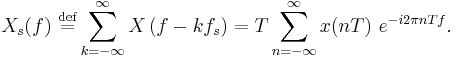
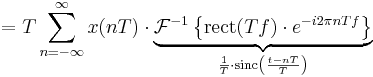
The Poisson summation formula indicates that the samples of function x(t) are sufficient to create a periodic extension of function X(f). The result is:
-
(
As depicted in Figures 3, 4, and 8, copies of X(f) are shifted by multiples of and combined by addition.

If the sampling condition is not satisfied, adjacent copies overlap, and it is not possible in general to discern an unambiguous X(f). Any frequency component above is indistinguishable from a lower-frequency component, called an alias, associated with one of the copies. The reconstruction technique described below produces the alias, rather than the original component, in such cases.

For a sinusoidal component of exactly half the sampling frequency, the component will in general alias to another sinusoid of the same frequency, but with a different phase and amplitude.
To prevent or reduce aliasing, two things can be done:
- Increase the sampling rate, to above twice some or all of the frequencies that are aliasing.
- Introduce an anti-aliasing filter or make the anti-aliasing filter more stringent.
The anti-aliasing filter is to restrict the bandwidth of the signal to satisfy the condition for proper sampling. Such a restriction works in theory, but is not precisely satisfiable in reality, because realizable filters will always allow some leakage of high frequencies. However, the leakage energy can be made small enough so that the aliasing effects are negligible.
Application to multivariable signals and images


The sampling theorem is usually formulated for functions of a single variable. Consequently, the theorem is directly applicable to time-dependent signals and is normally formulated in that context. However, the sampling theorem can be extended in a straightforward way to functions of arbitrarily many variables. Grayscale images, for example, are often represented as two-dimensional arrays (or matrices) of real numbers representing the relative intensities of pixels (picture elements) located at the intersections of row and column sample locations. As a result, images require two independent variables, or indices, to specify each pixel uniquely — one for the row, and one for the column.
Color images typically consist of a composite of three separate grayscale images, one to represent each of the three primary colors — red, green, and blue, or RGB for short. Other colorspaces using 3-vectors for colors include HSV, LAB, XYZ, etc. Some colorspaces such as cyan, magenta, yellow, and black (CMYK) may represent color by four dimensions. All of these are treated as vector-valued functions over a two-dimensional sampled domain.
Similar to one-dimensional discrete-time signals, images can also suffer from aliasing if the sampling resolution, or pixel density, is inadequate. For example, a digital photograph of a striped shirt with high frequencies (in other words, the distance between the stripes is small), can cause aliasing of the shirt when it is sampled by the camera's image sensor. The aliasing appears as a moiré pattern. The "solution" to higher sampling in the spatial domain for this case would be to move closer to the shirt, use a higher resolution sensor, or to optically blur the image before acquiring it with the sensor.
Another example is shown to the right in the brick patterns. The top image shows the effects when the sampling theorem's condition is not satisfied. When software rescales an image (the same process that creates the thumbnail shown in the lower image) it, in effect, runs the image through a low-pass filter first and then downsamples the image to result in a smaller image that does not exhibit the moiré pattern. The top image is what happens when the image is downsampled without low-pass filtering: aliasing results.
The top image was created by zooming out in GIMP and then taking a screenshot of it. The likely reason that this causes a banding problem is that the zooming feature simply downsamples without low-pass filtering (probably for performance reasons) since the zoomed image is for on-screen display instead of printing or saving.
The application of the sampling theorem to images should be made with care. For example, the sampling process in any standard image sensor (CCD or CMOS camera) is relatively far from the ideal sampling which would measure the image intensity at a single point. Instead these devices have a relatively large sensor area at each sample point in order to obtain sufficient amount of light. In other words, any detector has a finite-width point spread function. The analog optical image intensity function which is sampled by the sensor device is not in general bandlimited, and the non-ideal sampling is itself a useful type of low-pass filter, though not always sufficient to remove enough high frequencies to sufficiently reduce aliasing. When the area of the sampling spot (the size of the pixel sensor) is not large enough to provide sufficient anti-aliasing, a separate anti-aliasing filter (optical low-pass filter) is typically included in a camera system to further blur the optical image. Despite images having these problems in relation to the sampling theorem, the theorem can be used to describe the basics of down and up sampling of images.
Downsampling
When a signal is downsampled, the sampling theorem can be invoked via the artifice of resampling a hypothetical continuous-time reconstruction. The Nyquist criterion must still be satisfied with respect to the new lower sampling frequency in order to avoid aliasing. To meet the requirements of the theorem, the signal must usually pass through a low-pass filter of appropriate cutoff frequency as part of the downsampling operation. This low-pass filter, which prevents aliasing, is called an anti-aliasing filter.
Critical frequency

The Nyquist rate is defined as twice the bandwidth of the continuous-time signal. The sampling frequency must be strictly greater than the Nyquist rate of the signal to achieve unambiguous representation of the signal. This constraint is equivalent to requiring that the system's Nyquist frequency (also known as critical frequency, and equal to half the sample rate) be strictly greater than the bandwidth of the signal. If the signal contains a frequency component at precisely the Nyquist frequency then the corresponding component of the sample values cannot have sufficient information to reconstruct the Nyquist-frequency component in the continuous-time signal because of phase ambiguity. In such a case, there would be an infinite number of possible and different sinusoids (of varying amplitude and phase) of the Nyquist-frequency component that are represented by the discrete samples.
As an example, consider this family of signals at the critical frequency:
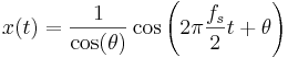
Where the samples
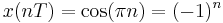
are in every case just alternating –1 and +1, for any phase θ. There is no way to determine either the amplitude or the phase of the continuous-time sinusoid x(t) that x(nT) was sampled from. This ambiguity is the reason for the strict inequality of the sampling theorem's condition.
Mathematical basis for the theorem

From Figures 3 and 8, it is apparent that when there is no overlap of the copies (aka "images") of X(f), the k=0 term of Xs(f) can be recovered by the product:
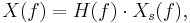 where:
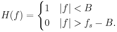
H(f) need not be precisely defined in the region [B, fs-B], because Xs(f) is zero in that region. However, the worst case is when B = fs/2, the Nyquist frequency. A function that is sufficient for that and all less severe cases is:
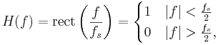
where  is the rectangular function.
Therefore:

-
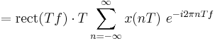 (from Eq.1 , above).
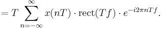
-
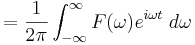
The original function that was sampled can be recovered by an inverse Fourier transform:


which is the Whittaker–Shannon interpolation formula. It shows explicitly how the samples, x(nT), can be combined to reconstruct x(t).
- From Figure 8, it is clear that larger-than-necessary values of fs (smaller values of T), called oversampling, have no effect on the outcome of the reconstruction and have the benefit of leaving room for a transition band in which H(f) is free to take intermediate values. Undersampling, which causes aliasing, is not in general a reversible operation.
- Theoretically, the interpolation formula can be implemented as a low pass filter, whose impulse response is
 and whose input is
 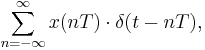 which is a Dirac comb function modulated by the signal samples. Practical digital-to-analog converters (DAC) implement an approximation like the zero-order hold. In that case, oversampling can reduce the approximation error.
Shannon's original proof
The original proof presented by Shannon is elegant and quite brief, but it offers less intuitive insight into the subtleties of aliasing, both unintentional and intentional. Quoting Shannon's original paper, which uses f for the function, F for the spectrum, and W for the bandwidth limit:
- Let
 be the spectrum of
  . Then

- since is assumed to be zero outside the band W. If we let

- where n is any positive or negative integer, we obtain
- On the left are values of at the sampling points. The integral on the right will be recognized as essentially the nth coefficient in a Fourier-series expansion of the function , taking the interval –W to W as a fundamental period. This means that the values of the samples
 determine the Fourier coefficients in the series expansion of . Thus they determine , since is zero for frequencies greater than W, and for lower frequencies is determined if its Fourier coefficients are determined. But determines the original function completely, since a function is determined if its spectrum is known. Therefore the original samples determine the function completely.
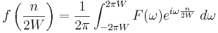
Shannon's proof of the theorem is complete at that point, but he goes on to discuss reconstruction via sinc functions, what we now call the Whittaker–Shannon interpolation formula as discussed above. He does not derive or prove the properties of the sinc function, but these would have been familiar to engineers reading his works at the time, since the Fourier pair relationship between rect and sinc was well known. Quoting Shannon:
- Let
 be the nth sample. Then the function is represented by:

As in the other proof, the existence of the Fourier transform of the original signal is assumed, so the proof does not say whether the sampling theorem extends to bandlimited stationary random processes.
Sampling of non-baseband signals
For sampling a non-baseband signal, the conditions to avoid information loss and to allow perfect reconstruction can be generalized in terms of conditions on the frequency interval of nonzero spectrum. See Sampling (signal processing) for more details and examples.
A bandpass condition is that  for all nonnegative
  outside the open band of frequencies:

for some nonnegative integer  . This formulation includes the normal baseband condition as the case N=0.
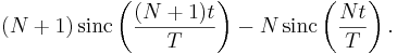
The corresponding interpolation function is the impulse response of a bandpass filter with cutoffs at the upper and lower edges of the specified band, which is the difference between a pair of lowpass impulse responses:
Other generalizations, for example to signals occupying multiple non-contiguous bands, are possible as well. Even the most generalized form of the sampling theorem does not have a provably true converse. That is, one cannot conclude that information is necessarily lost just because the conditions of the sampling theorem are not satisfied; from an engineering perspective, however, it is generally safe to assume that if the sampling theorem is not satisfied then information will most likely be lost.
Nonuniform sampling
The sampling theory of Shannon can be generalized for the case of nonuniform samples, that is, samples not taken equally spaced in time. Shannon sampling theory for non-uniform sampling states that a band-limited signal can be perfectly reconstructed from its samples if the average sampling rate satisfies the Nyquist condition[3]. Therefore, although uniformly spaced samples may result in easier reconstruction algorithms, it is not a necessary condition for perfect reconstruction.
Historical background
The sampling theorem was implied by the work of Harry Nyquist in 1928 ("Certain topics in telegraph transmission theory"), in which he showed that up to 2B independent pulse samples could be sent through a system of bandwidth B; but he did not explicitly consider the problem of sampling and reconstruction of continuous signals. About the same time, Karl Küpfmüller showed a similar result[4], and discussed the sinc-function impulse response of a band-limiting filter, via its integral, the step response Integralsinus; this bandlimiting and reconstruction filter that is so central to the sampling theorem is sometimes referred to as a Küpfmüller filter (but seldom so in English).
The sampling theorem, essentially a dual of Nyquist's result, was proved by Claude E. Shannon in 1949 ("Communication in the presence of noise"). V. A. Kotelnikov published similar results in 1933 ("On the transmission capacity of the 'ether' and of cables in electrical communications", translation from the Russian), as did the mathematician E. T. Whittaker in 1915 ("Expansions of the Interpolation-Theory", "Theorie der Kardinalfunktionen"), J. M. Whittaker in 1935 ("Interpolatory function theory"), and Gabor in 1946 ("Theory of communication").
Other discoverers
Others who have independently discovered or played roles in the development of the sampling theorem have been discussed in several historical articles, for example by Jerri[5] and by Lüke.[6] For example, Lüke points out that H. Raabe, an assistant to Küpfmüller, proved the theorem in his 1939 Ph.D. dissertation; the term Raabe condition came to be associated with the criterion for unambiguous representation (sampling rate greater than twice the bandwidth).
Meijering[7] mentions several other discoverers and names in a paragraph and pair of footnotes:
As pointed out by Higgins [135], the sampling theorem should really be considered in two parts, as done above: the first stating the fact that a bandlimited function is completely determined by its samples, the second describing how to reconstruct the function using its samples. Both parts of the sampling theorem were given in a somewhat different form by J. M. Whittaker [350, 351, 353] and before him also by Ogura [241, 242]. They were probably not aware of the fact that the first part of the theorem had been stated as early as 1897 by Borel [25].27 As we have seen, Borel also used around that time what became known as the cardinal series. However, he appears not to have made the link [135]. In later years it became known that the sampling theorem had been presented before Shannon to the Russian communication community by Kotel'nikov [173]. In more implicit, verbal form, it had also been described in the German literature by Raabe [257]. Several authors [33, 205] have mentioned that Someya [296] introduced the theorem in the Japanese literature parallel to Shannon. In the English literature, Weston [347] introduced it independently of Shannon around the same time.28
27 Several authors, following Black [16], have claimed that this first part of the sampling theorem was stated even earlier by Cauchy, in a paper [41] published in 1841. However, the paper of Cauchy does not contain such a statement, as has been pointed out by Higgins [135].
28 As a consequence of the discovery of the several independent introductions of the sampling theorem, people started to refer to the theorem by including the names of the aforementioned authors, resulting in such catchphrases as “the Whittaker-Kotel’nikov-Shannon (WKS) sampling theorem" [155] or even "the Whittaker-Kotel'nikov-Raabe-Shannon-Someya sampling theorem" [33]. To avoid confusion, perhaps the best thing to do is to refer to it as the sampling theorem, "rather than trying to find a title that does justice to all claimants" [136].
Why Nyquist?
Exactly how, when, or why Harry Nyquist had his name attached to the sampling theorem remains obscure. The term Nyquist Sampling Theorem (capitalized thus) appeared as early as 1959 in a book from his former employer, Bell Labs,[8] and appeared again in 1963,[9] and not capitalized in 1965.[10] It had been called the Shannon Sampling Theorem as early as 1954,[11] but also just the sampling theorem by several other books in the early 1950s.
In 1958, Blackman and Tukey[12] cited Nyquist's 1928 paper as a reference for the sampling theorem of information theory, even though that paper does not treat sampling and reconstruction of continuous signals as others did. Their glossary of terms includes these entries:
- Sampling theorem (of information theory)
- Nyquist's result that equi-spaced data, with two or more points per cycle of highest frequency, allows reconstruction of band-limited functions. (See Cardinal theorem.)
- Cardinal theorem (of interpolation theory)
- A precise statement of the conditions under which values given at a doubly infinite set of equally spaced points can be interpolated to yield a continuous band-limited function with the aid of the function

Exactly what "Nyquist's result" they are referring to remains mysterious.
When Shannon stated and proved the sampling theorem in his 1949 paper, according to Meijering[7] "he referred to the critical sampling interval T = 1/2W as the Nyquist interval corresponding to the band W, in recognition of Nyquist’s discovery of the fundamental importance of this interval in connection with telegraphy." This explains Nyquist's name on the critical interval, but not on the theorem.
Similarly, Nyquist's name was attached to Nyquist rate in 1953 by Harold S. Black:[13]
- "If the essential frequency range is limited to B cycles per second, 2B was given by Nyquist as the maximum number of code elements per second that could be unambiguously resolved, assuming the peak interference is less half a quantum step. This rate is generally referred to as signaling at the Nyquist rate and 1/2B has been termed a Nyquist interval." (bold added for emphasis; italics as in the original)
According to the OED, this may be the origin of the term Nyquist rate. In Black's usage, it is not a sampling rate, but a signaling rate.
Notes
- ↑ C. E. Shannon, "Communication in the presence of noise", Proc. Institute of Radio Engineers, vol. 37, no.1, pp. 10-21, Jan. 1949. Reprint as classic paper in: Proc. IEEE, Vol. 86, No. 2, (Feb 1998)
- ↑ The time-domain form follows from rows 202 and 102 of the transform tables
- ↑ Nonuniform Sampling, Theory and Practice (ed. F. Marvasti), Kluwer Academic/Plenum Publishers, New York, 2000
- ↑ K. Küpfmüller, "Über die Dynamik der selbsttätigen Verstärkungsregler", Elektrische Nachrichtentechnik, vol. 5, no. 11, pp. 459-467, 1928. (German)
K. Küpfmüller, On the dynamics of automatic gain controllers, Elektrische Nachrichtentechnik, vol. 5, no. 11, pp. 459-467. (English translation) - ↑ Abdul Jerri, The Shannon Sampling Theorem—Its Various Extensions and Applications: A Tutorial Review, Proceedings of the IEEE, 65:1565–1595, Nov. 1977. See also Correction to "The Shannon sampling theorem—Its various extensions and applications: A tutorial review", Proceedings of the IEEE, 67:695, April 1979
- ↑ Hans Dieter Lüke, The Origins of the Sampling Theorem , IEEE Communications Magazine, pp.106–108, April 1999.
- ↑ 7.0 7.1 Erik Meijering, A Chronology of Interpolation From Ancient Astronomy to Modern Signal and Image Processing , Proc. IEEE, 90, 2002.
- ↑ Members of the Technical Staff of Bell Telephone Lababoratories (1959). Transmission Systems for Communications. AT&T. pp. 26–4 (Vol.2).
- ↑ Ernst Adolph Guillemin (1963). Theory of Linear Physical Systems. Wiley. http://books.google.com/books?id=jtI-AAAAIAAJ&q=Nyquist-sampling-theorem+date:0-1965&dq=Nyquist-sampling-theorem+date:0-1965&as_brr=0&ei=ief5Ru-DJqegowLyiJTpBw&pgis=1.
- ↑ Richard A. Roberts and Ben F. Barton, Theory of Signal Detectability: Composite Deferred Decision Theory, 1965.
- ↑ Truman S. Gray, Applied Electronics: A First Course in Electronics, Electron Tubes, and Associated Circuits, 1954.
- ↑ R. B. Blackman and J. W. Tukey, The Measurement of Power Spectra : From the Point of View of Communications Engineering, New York: Dover, 1958.
- ↑ Harold S. Black, Modulation Theory, 1953
Other references
- E. T. Whittaker, "On the Functions Which are Represented by the Expansions of the Interpolation Theory", Proc. Royal Soc. Edinburgh, Sec. A, vol.35, pp.181-194, 1915
- H. Nyquist, "Certain topics in telegraph transmission theory", Trans. AIEE, vol. 47, pp. 617-644, Apr. 1928 Reprint as classic paper in: Proc. IEEE, Vol. 90, No. 2, Feb 2002.
- Karl Küpfmüller, "Utjämningsförlopp inom Telegraf- och Telefontekniken", ("Transients in telegraph and telephone engineering"), Teknisk Tidskrift, no. 9 pp.153-160 and 10 pp.178-182, 1931. [1] [2]
- V. A. Kotelnikov, "On the carrying capacity of the ether and wire in telecommunications", Material for the First All-Union Conference on Questions of Communication, Izd. Red. Upr. Svyazi RKKA, Moscow, 1933 (Russian). (english translation, PDF)
- J. M. Whittaker, Interpolatory Function Theory, Cambridge Univ. Press, Cambridge, England, 1935.
- C. E. Shannon, "Communication in the presence of noise", Proc. Institute of Radio Engineers, vol. 37, no.1, pp. 10-21, Jan. 1949. Reprint as classic paper in: Proc. IEEE, Vol. 86, No. 2, (Feb 1998)
- J. R. Higgins: Five short stories about the cardinal series, Bulletin of the AMS 12(1985)
- Michael Unser: Sampling-50 Years after Shannon, Proc. IEEE, vol. 88, no. 4, pp. 569-587, April 2000
See also
- Aliasing
- Anti-aliasing filter
- Dirac comb
- Nyquist rate - a maximum baud rate
- Hartley's law - a maximum bit rate based on the sampling theorem.
- Whittaker–Shannon interpolation formula
- Sampling (signal processing)
- Signal (electrical engineering)
- Reconstruction from zero crossings
External links
- Learning by Simulations Interactive simulation of the effects of inadequate sampling
- Undersampling and an application of it
- Sampling Theory For Digital Audio
- Journal devoted to Sampling Theory
|
||||||||||||||
|
|||||||||||||||||||||||||||||||||||||||||||||||||||||||