Nash equilibrium

Nash Equilibrium
A solution concept in game theory
Relationships
Subset of:	Rationalizability, Epsilon-equilibrium, Correlated equilibrium
Superset of:	Evolutionarily stable strategy, Subgame perfect equilibrium, Perfect Bayesian equilibrium, Trembling hand perfect equilibrium
Significance
Proposed by:	John Forbes Nash
Used for:	All non-cooperative games
Example:	Rock paper scissors

In game theory, Nash equilibrium (named after John Forbes Nash, who proposed it) is a solution concept of a game involving two or more players, in which each player is assumed to know the equilibrium strategies of the other players, and no player has anything to gain by changing only his or her own strategy (i.e., by changing unilaterally). If each player has chosen a strategy and no player can benefit by changing his or her strategy while the other players keep theirs unchanged, then the current set of strategy choices and the corresponding payoffs constitute a Nash equilibrium. In other words, to be in a Nash equilibrium, each player must answer negatively to the question: "Knowing the strategies of the other players, and treating the strategies of the other players as set in stone, can I benefit by changing my strategy?"

Stated simply, Amy and Bill are in Nash equilibrium if Amy is making the best decision she can, taking into account Bill's decision, and Bill is making the best decision he can, taking into account Amy's decision. Likewise, many players are in Nash equilibrium if each one is making the best decision that they can, taking into account the decisions of the others. However, Nash equilibrium does not necessarily mean the best cumulative payoff for all the players involved; in many cases all the players might improve their payoffs if they could somehow agree on strategies different from the Nash equilibrium (e.g. competing businessmen forming a cartel in order to increase their profits).

History

The concept of the Nash equilibrium (NE) in pure strategies was first developed by Antoine Augustin Cournot in his theory of oligopoly (1838). Firms choose a quantity of output to maximize their own profit. However, the best output for one firm depends on the outputs of others. A Cournot equilibrium occurs when each firm's output maximizes its profits given the output of the other firms, which is a pure-strategy NE. However, the modern game-theoretic concept of NE is defined in terms of mixed-strategies, where players choose a probability distribution over possible actions. The concept of the mixed strategy NE was introduced by John von Neumann and Oskar Morgenstern in their 1944 book The Theory of Games and Economic Behavior. However, their analysis was restricted to the very special case of zero-sum games. They showed that a mixed-strategy NE will exist for any zero-sum game with a finite set of actions. The contribution of John Forbes Nash in his 1951 article Non-Cooperative Games was to define a mixed strategy NE for any game with a finite set of actions and prove that at least one (mixed strategy) NE must exist.

Definitions

Informal definition

Informally, a set of strategies is a Nash equilibrium if no player can do better by unilaterally changing his or her strategy. As a heuristic, one can imagine that each player is told the strategies of the other players. If any player would want to do something different after being informed about the others' strategies, then that set of strategies is not a Nash equilibrium. If, however, the player does not want to switch (or is indifferent between switching and not) then the set of strategies is a Nash equilibrium.

Each strategy in a Nash equilibrium is a best response to all other strategies in that equilibrium.^[1]

The Nash equilibrium may sometimes appear non-rational in a third-person perspective. This is because it may happen that a Nash equilibrium is not pareto optimal.

The Nash equilibrium may also have non-rational consequences in sequential games because players may "threat"-en each other with non-rational moves. For such games the Subgame perfect Nash equilibrium may be more meaningful as a tool of analysis.

Formal definition

Let (S, f) be a game, where S_i is the strategy set for player i, S=S₁ X S₂ ... X S_n is the set of strategy profiles and f=(f₁(x), ..., f_n(x)) is the payoff function. Let $x_{-i}$ be a strategy profile of all players except for player i. When each player i $\in$ {1, ..., n} chooses strategy x_i resulting in strategy profile x = (x₁, ..., x_n) then player i obtains payoff f_i(x). Note that the payoff depends on the strategy profile chosen, i.e. on the strategy chosen by player i as well as the strategies chosen by all the other players. A strategy profile x^* $\in$ S is a Nash equilibrium (NE) if no unilateral deviation in strategy by any single player is profitable for that player, that is

$\forall i,x_i\in S_i, x_i \neq x^*_{i}�: f_i(x^*_{i}, x^*_{-i}) \geq f_i(x_{i},x^*_{-i}).$

A game can have a pure strategy NE or an NE in its mixed extension (that of choosing a pure strategy stochastically with a fixed frequency). Nash proved that if we allow mixed strategies, then every n-player game in which every player can choose from finitely many strategies admits at least one Nash equilibrium.

When the inequality above holds strictly (with $>$ instead of $\geq$ ) for all players and all feasible alternative strategies, then the equilibrium is classified as a strict Nash equilibrium. If instead, for some player, there is exact equality between $x^*_i$ and some other strategy in the set $S$ , then the equilibrium is classified as a weak Nash equilibrium.

Examples

Competition game

*A competition game*
	Player 2 chooses '0'	Player 2 chooses '1'	Player 2 chooses '2'	Player 2 chooses '3'
Player 1 chooses '0'	0, 0	2, -2	2, -2	2, -2
Player 1 chooses '1'	-2, 2	1, 1	3, -1	3, -1
Player 1 chooses '2'	-2, 2	-1, 3	2, 2	4, 0
Player 1 chooses '3'	-2, 2	-1, 3	0, 4	3, 3

This can be illustrated by a two-player game in which both players simultaneously choose a whole number from 0 to 3 and they both win the smaller of the two numbers in points. In addition, if one player chooses a larger number than the other, then he/she has to give up two points to the other. This game has a unique pure-strategy Nash equilibrium: both players choosing 0 (highlighted in light red). Any other choice of strategies can be improved if one of the players lowers his number to one less than the other player's number. In the table to the left, for example, when starting at the green square it is in player 1's interest to move to the purple square by choosing a smaller number, and it is in player 2's interest to move to the blue square by choosing a smaller number. If the game is modified so that the two players win the named amount if they both choose the same number, and otherwise win nothing, then there are 4 Nash equilibria (0,0...1,1...2,2...and 3,3).

Coordination game

Main article: Coordination game

*A coordination game*
	Player 2 adopts strategy 1	Player 2 adopts strategy 2
Player 1 adopts strategy 1	A, A	B, C
Player 1 adopts strategy 2	C, B	D, D

The coordination game is a classic (symmetric) two player, two strategy game, with the payoff matrix shown to the right, where the payoffs satisfy A>C and D>B. The players should thus coordinate, either on A or on D, to receive a high payoff. If the players' choices do not coincide, a lower payoff is rewarded. An example of a coordination game is the setting where two technologies are available to two firms with compatible products, and they have to elect a strategy to become the market standard. If both firms agree on the chosen technology, high sales are expected for both firms. If the firms do not agree on the standard technology, few sales result. Both strategies are Nash equilibria of the game.

Driving on a road, and having to choose either to drive on the left or to drive on the right of the road, is also a coordination game. For example, with payoffs 100 meaning no crash and 0 meaning a crash, the coordination game can be defined with the following payoff matrix:

*The driving game*
	Drive on the Left	Drive on the Right
Drive on the Left	100, 100	0, 0
Drive on the Right	0, 0	100, 100

In this case there are two pure strategy Nash equilibria, when both choose to either drive on the left or on the right. If we admit mixed strategies (where a pure strategy is chosen at random, subject to some fixed probability), then there are three Nash equilibria for the same case: two we have seen from the pure-strategy form, where the probabilities are (0%,100%) for player one, (0%, 100%) for player two; and (100%, 0%) for player one, (100%, 0%) for player two respectively. We add another where the probabilities for each player is (50%, 50%).

Prisoner's dilemma

Main article: Prisoner's dilemma

(note differences in the orientation of the payoff matrix)

The Prisoner's Dilemma has the same payoff matrix as depicted for the Coordination Game, but now C > A > D > B. Because C > A and D > B, each player improves his situation by switching from strategy #1 to strategy #2, no matter what the other player decides. The Prisoner's Dilemma thus has a single Nash Equilibrium: both players choosing strategy #2 ("betraying"). What has long made this an interesting case to study is the fact that D < A (ie., "both betray" is globally inferior to "both remain loyal"). The globally optimal strategy is unstable; it is not an equilibrium.

Nash equilibria in a payoff matrix

There is an easy numerical way to identify Nash Equilibria on a Payoff Matrix. It is especially helpful in two-person games where players have more than two strategies. In this case formal analysis may become too long. This rule does not apply to the case where mixed (stochastic) strategies are of interest. The rule goes as follows: if the first payoff number, in the duplet of the cell, is the maximum of the column of the cell and if the second number is the maximum of the row of the cell - then the cell represents a Nash equilibrium.

We can apply this rule to a 3x3 matrix:

*A Payoff Matrix*
	Option A	Option B	Option C
Option A	0, 0	25, 40	5, 10
Option B	40, 25	0, 0	5, 15
Option C	10, 5	15, 5	10, 10

Using the rule, we can very quickly (much faster than with formal analysis) see that the Nash Equlibria cells are (B,A), (A,B), and (C,C). Indeed, for cell (B,A) 40 is the maximum of the first column and 25 is the maximum of the second row. For (A,B) 25 is the maximum of the second column and 40 is the maximum of the first row. Same for cell (C,C). For other cells, either one or both of the duplet members are not the maximum of the corresponding rows and columns.

This said, the actual mechanics of finding equilibrium cells is obvious: find the maximum of a column and check if the second member of the pair is the maximum of the row. If these conditions are met, the cell represents a Nash Equilibrium. Check all columns this way to find all NE cells. An NxN matrix may have between 0 and NxN pure strategy Nash equilibria.

Network traffic

See also: Braess's Paradox

Sample network graph. Values on edges are the travel time experienced by a 'car' travelling down that edge. X is the number of cars travelling via that edge.

An extension of Nash equilibria is in determining the expected flow of traffic in a network. Consider the graph on the right. If we assume that there are $n$ "cars" traveling from A to D, what is the expected distribution of traffic in the network?

This situation can be modeled as a "game" where every traveler has a choice of 3 strategies, where each strategy is a route from A to D (either $ABD$ , $ABCD$ , or $ACD$ ). The "payoff" of each strategy is the travel time of each route. In the graph on the right, a car travelling via $ABD$ experiences travel time of $(1+x/100+2$ , where $x$ is the number of cars traveling on edge $AB$ . Thus, payoffs for any given strategy depend on the choices of the other players, as is usual. However, the goal in this case is to minimize travel time, not maximize it. Equilibrium will occur when the time on all paths is exactly the same. When that happens, no single driver has any incentive to switch routes, since it can only add to his/her travel time. For the graph on the right, if, for example, 100 cars are travelling from A to D, then equilibrium will occur when 25 drivers travel via $ABD$ , 50 via $ABCD$ , and 25 via $ACD$ . Every driver now has a total travel time of 3.75.

Notice that this distribution is not, actually, socially optimal. If the 100 cars agreed that 50 travel via $ABD$ and the other 50 through $ACD$ , then travel time for any single car would actually be 3.5, which is less than 3.75.

Stability

The concept of stability, useful in the analysis of many kinds of equilibrium, can also be applied to Nash equilibria.

A Nash equilibrium for a mixed strategy game is stable if a small change (specifically, an infinitesimal change) in probabilities for one player leads to a situation where two conditions hold:

the player who did not change has no better strategy in the new circumstance
the player who did change is now playing with a strictly worse strategy

If these cases are both met, then a player with the small change in his mixed-strategy will return immediately to the Nash equilibrium. The equilibrium is said to be stable. If condition one does not hold then the equilibrium is unstable. If only condition one holds then there are likely to be an infinite number of optimal strategies for the player who changed. John Nash showed that the latter situation could not arise in a range of well-defined games.

In the "driving game" example above there are both stable and unstable equilibria. The equilibria involving mixed-strategies with 100% probabilities are stable. If either player changes his probabilities slightly, they will be both at a disadvantage, and his opponent will have no reason to change his strategy in turn. The (50%,50%) equilibrium is unstable. If either player changes his probabilities, then the other player immediately has a better strategy at either (0%, 100%) or (100%, 0%).

Stability is crucial in practical applications of Nash equilibria, since the mixed-strategy of each player is not perfectly known, but has to be inferred from statistical distribution of his actions in the game. In this case unstable equilibria are very unlikely to arise in practice, since any minute change in the proportions of each strategy seen will lead to a change in strategy and the breakdown of the equilibrium.

A Coalition-Proof Nash Equilibrium (CPNE) (similar to a Strong Nash Equilibrium) occurs when players cannot do better even if they are allowed to communicate and collaborate before the game. Every correlated strategy supported by iterated strict dominance and on the Pareto frontier is a CPNE^[2]. Further, it is possible for a game to have a Nash equilibrium that is resilient against coalitions less than a specified size, k. CPNE is related to the theory of the core.

Occurrence

If a game has a unique Nash equilibrium and is played among players under certain conditions, then the NE strategy set will be adopted. Sufficient conditions to guarantee that the Nash equilibrium is played are:

The players all will do their utmost to maximize their expected payoff as described by the game.
The players are flawless in execution.
The players have sufficient intelligence to deduce the solution.
The players know the planned equilibrium strategy of all of the other players.
The players believe that a deviation in their own strategy will not cause deviations by any other players.
There is common knowledge that all players meet these conditions, including this one. So, not only must each player know the other players meet the conditions, but also they must know that they all know that they meet them, and know that they know that they know that they meet them, and so on.

Where the conditions are not met

Examples of game theory problems in which these conditions are not met:

The first condition is not met if the game does not correctly describe the quantities a player wishes to maximize. In this case there is no particular reason for that player to adopt an equilibrium strategy. For instance, the prisoner’s dilemma is not a dilemma if either player is happy to be jailed indefinitely.
Intentional or accidental imperfection in execution. For example, a computer capable of flawless logical play facing a second flawless computer will result in equilibrium. Introduction of imperfection will lead to its disruption either through loss to the player who makes the mistake, or through negation of the 4th 'common knowledge' criterion leading to possible victory for the player. (An example would be a player suddenly putting the car into reverse in the game of 'chicken', ensuring a no-loss no-win scenario).
In many cases, the third condition is not met because, even though the equilibrium must exist, it is unknown due to the complexity of the game, for instance in Chinese chess.^[3] Or, if known, it may not be known to all players, as when playing tic-tac-toe with a small child who desperately wants to win (meeting the other criteria).
The fourth criterion of common knowledge may not be met even if all players do, in fact, meet all the other criteria. Players wrongly distrusting each other's rationality may adopt counter-strategies to expected irrational play on their opponents’ behalf. This is a major consideration in “Chicken” or an arms race, for example.

Where the conditions are met

Due to the limited conditions in which NE can actually be observed, they are rarely treated as a guide to day-to-day behaviour, or observed in practice in human negotiations. However, as a theoretical concept in economics, and evolutionary biology the NE has explanatory power. The payoff in economics is money, and in evolutionary biology gene transmission, both are the fundamental bottom line of survival. Researchers who apply games theory in these fields claim that agents failing to maximize these for whatever reason will be competed out of the market or environment, which are ascribed the ability to test all strategies. This conclusion is drawn from the "stability" theory above. In these situations the assumption that the strategy observed is actually a NE has often been borne out by research.

NE and non-credible threats

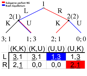
Extensive and Normal form illustrations that show the difference between SPNE and other NE. The blue equilibrium is not subgame perfect because player two makes a non-credible threat at 2(2) to be unkind (U).

The nash equilibrium is a superset of the subgame perfect nash equilibrium. The subgame perfect equilibrium in addition to the Nash Equilibrium requires that the strategy also is a Nash equilibrium in every subgame of that game. This eliminates all non-credible threats, that is, strategies that contain non-rational moves in order to make the counter-player change his strategy.

The image to the right shows a simple sequential game that illustrates the issue with subgame imperfect Nash equilibria. In this game player one chooses left(L) or right(R), which is followed by player two being called upon to be kind (K) or unkind (U) to player one, However, player two only stands to gain from being unkind if player one goes left. If player one goes right the rational player two would de facto be kind to him in that subgame. However, The non-credible threat of being unkind at 2(2) is still part of the blue (L, (U,U)) nash equilibrium. Therefore, if rational behavior can be expected by both parties the subgame perfect Nash equilibrium may be a more meaningful solution concept when such dynamic inconsistencies arise.

Proof of existence

As above, let $\sigma_{-i}$ be a mixed strategy profile of all players except for player $i$ . We can define a best response correspondence for player $i$ , $b_i$ . $b_i$ is a relation from the set of all probability distributions over opponent player profiles to a set of player $i$ 's strategies, such that each element of

$b_i(\sigma_{-i})$

is a best response to $\sigma_{-i}$ . Define

$b(\sigma) = b_1(\sigma_{-1}) \times b_2(\sigma_{-2}) \times \cdots \times b_n(\sigma_{-n})$ .

One can use the Kakutani fixed point theorem to prove that $b$ has a fixed point. That is, there is a $\sigma^*$ such that $\sigma^* \in b(\sigma^*)$ . Since $b(\sigma^*)$ represents the best response for all players to $\sigma^*$ , the existence of the fixed point proves that there is some strategy set which is a best response to itself. No player could do any better by deviating, and it is therefore a Nash equilibrium.

When Nash made this point to John von Neumann in 1949, von Neumann famously dismissed it with the words, "That's trivial, you know. That's just a fixed point theorem." (See Nasar, 1998, p. 94.)

Alternate proof using the Brouwer fixed point theorem

We have a game $G=(N,A,u)$ where $N$ is the number of players and $A = A_1 \times \ldots \times A_N$ is the action set for the players. All of the actions sets $A_i$ are finite. Let $\Delta = \Delta_1 \times \ldots \times \Delta_N$ denote the set of mixed strategies for the players. The finiteness of the $A_i$ s insures the compactness of $\Delta$ .

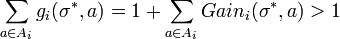
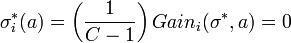
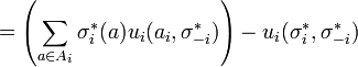
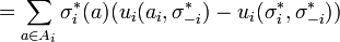
We can now define the gain functions. For a mixed strategy $\sigma \in \Delta$ , we let the gain for player $i$ on action $a \in A_i$ be

$Gain_i(\sigma,a) = \max \{0, u_i(a_i, \sigma_{-i}) - u_i(\sigma_{i}, \sigma_{-i})\}$

The gain function represents the benefit a player gets by unilaterally changing his strategy. We now define $g = (g_1,\ldots,g_N)$ where

$g_i(\sigma)(a) = \sigma_i(a) + Gain_i(\sigma,a)$

for $\sigma \in \Delta, a \in A_i$ . We see that

$\sum_{a \in A_i} g_i(\sigma)(a) = \sum_{a \in A_i} \sigma_i(a) + Gain_i(\sigma,a) = 1 + \sum_{a \in A_i} Gain_i(\sigma,a) > 0$

We now use $g$ to define $f: \Delta \rightarrow \Delta$ as follows. Let

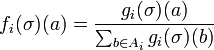
$f_i(\sigma)(a) = \frac{g_i(\sigma)(a)}{\sum_{b \in A_i} g_i(\sigma)(b)}$

for $a \in A_i$ . It is easy to see that each $f_i$ is a valid mixed strategy in $\Delta_i$ . It is also easy to check that each $f_i$ is a continuous function of $\sigma$ , and hence $f$ is a continuous function. Now $\Delta$ is the cross product of a finite number of compact convex sets, and so we get that $\Delta$ is also compact and convex. Therefore we may apply the Brouwer fixed point theorem to $f$ . So $f$ has a fixed point in $\Delta$ , call it $\sigma^*$ .

I claim that $\sigma^*$ is a Nash Equilibrium in $G$ . For this purpose, it suffices to show that

$\forall 1 \leq i \leq N, ~ \forall a \in A_i, ~ Gain_i(\sigma^*,a) = 0 \text{.}$

This simply states the each player gains no benefit by unilaterally changing his strategy which is exactly the necessary condition for being a Nash Equilibrium.

Now assume that the gains are not all zero. Therefore, $\exists i$ , $1 \leq 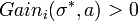i \leq N$ , and $a \in A_i$ such that $Gain_i(\sigma^*, a) > 0$ . Note then that

$\sum_{a \in A_i} g_i(\sigma^*, a) = 1 + \sum_{a \in A_i} Gain_i(\sigma^*,a) > 1$

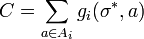So let $C = \sum_{a \in A_i} g_i(\sigma^*, a)$ . Also we shall denote $Gain(i,\cdot)$ as the gain vector indexed by actions in $A_i$ . Since $f(\sigma^*) = \sigma^*$ we clearly have that $f_i(\sigma^*) = \sigma^*_i$ . Therefore we see that

$\sigma^*_i = \frac{g_i(\sigma^*)}{\sum_{a \in A_i} g_i(\sigma^*)(a)} \Rightarrow \sigma^*_i = \frac{\sigma^*_i + Gain_i(\sigma^*,\cdot)}{C} \Rightarrow C\sigma^*_i = \sigma^*_i + Gain_i(\sigma^*,\cdot)$

$\left(C-1\right)\sigma^*_i = Gain_i(\sigma^*,\cdot) \Rightarrow \sigma^*_i = \left(\frac{1}{C-1}\right)Gain_i(\sigma^*,\cdot)$

Since $C > 1$ we have that $\sigma^*_i$ is some positive scaling of the vector $Gain_i(\sigma^*,\cdot)$ . Now I claim that

$\sigma^*_i(a)(u_i(a_i, \sigma^*_{-i}) - u_i(\sigma^*_i, \sigma^*_{-i})) = \sigma^*_i(a)Gain_i(\sigma^*, a)$

$\forall a \in A_i$ . To see this, we first note that if $Gain_i(\sigma^*, a) > 0$ then this is true by definition of the gain function. Now assume that 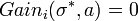$Gain_i(\sigma^*, a) = 0$ . By our previous statements we have that

$\sigma^*_i(a) = \left(\frac{1}{C-1}\right)Gain_i(\sigma^*, a) = 0$

and so the left term is zero, giving us that the entire expression is $0$ as needed.

So we finally have that

$0 = u_i(\sigma^*_i, \sigma^*_{-i}) - u_i(\sigma^*_i, \sigma^*_{-i})$

$= \left(\sum_{a \in A_i} \sigma^*_i(a)u_i(a_i, \sigma^*_{-i})\right) - u_i(\sigma^*_i, \sigma^*_{-i})$

$= \sum_{a \in A_i} \sigma^*_i(a) (u_i(a_i, \sigma^*_{-i}) - u_i(\sigma^*_i, \sigma^*_{-i}))$

$= \sum_{a \in A_i} \sigma^*_i(a) Gain_i(\sigma^*, a) \quad \text{ by the previous statements }$

$= \sum_{a \in A_i} \left( C -1 \right) \sigma^*_i(a)^2 > 0$

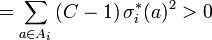
where the last inequality follows since $\sigma^*_i$ is a non-zero vector. But this is a clear contradiction, so all the gains must indeed be zero. Therefore $\sigma^*$ is a Nash Equilibrium for $G$ as needed.

Computing Nash equilibria

If a player A has a dominant strategy $s_A$ then there exists a Nash equilibrium in which A plays $s_A$ . In the case of two players A and B, there exists a Nash equilibrium in which A plays $s_A$ and B plays a best response to $s_A$ . If $s_A$ is a strictly dominant strategy, A plays $s_A$ in all Nash equilibria. If both A and B have strictly dominant strategies, there exists a unique Nash equilibrium in which each plays his strictly dominant strategy.

In games with mixed strategy Nash equilibria, the probability of a player choosing any particular strategy can be computed by assigning a variable to each strategy that represents a fixed probability for choosing that strategy. In order for a player to be willing to randomize, his expected payoff for each strategy should be the same. In addition, the sum of the probabilities for each strategy of a particular player should be 1. This creates a system of equations from which the probabilities of choosing each strategy can be derived.^[1]

Examples

*Matching pennies*
	Player A plays H	Player A plays T
Player B plays H	-1, +1	+1, -1
Player B plays T	+1, -1	-1, +1

In the matching pennies game, player A loses a point to B if A and B play the same strategy and wins a point from B if they play different strategies. To compute the mixed strategy Nash equilibrium, assign A the probability p of playing H and (1-p) of playing T, and assign B the probability q of playing H and (1-q) of playing T.

E[payoff for A playing H] = (-1)q + (+1)(1-q) = 1-2q
E[payoff for A playing T] = (+1)q + (-1)(1-q) = 2q-1
E[payoff for A playing H] = E[payoff for A playing T] ⇒ 1-2q = 2q-1 ⇒ q = 1/2

E[payoff for B playing H] = (+1)p + (-1)(1-p) = 2p-1
E[payoff for B playing T] = (-1)p + (+1)(1-p) = 1-2p
E[payoff for B playing H] = E[payoff for B playing T] ⇒ 2p-1 = 1-2p ⇒ p = 1/2

Thus a mixed strategy Nash equilibrium in this game is for each player to randomly choose H or T with equal probability.

References

Game Theory textbooks

Dutta, Prajit K. (1999), Strategies and games: theory and practice, MIT Press, ISBN 978-0-262-04169-0 . Suitable for undergraduate and business students.

Fudenberg, Drew and Jean Tirole (1991) Game Theory MIT Press.

Morgenstern, Oskar and John von Neumann (1947) The Theory of Games and Economic Behavior Princeton University Press

Myerson, Roger B. (1997), Game theory: analysis of conflict, Harvard University Press, ISBN 978-0-674-34116-6

Rubinstein, Ariel; Osborne, Martin J. (1994), A course in game theory, MIT Press, ISBN 978-0-262-65040-3 . A modern introduction at the graduate level.

Original Papers

Nash, John (1950) "Equilibrium points in n-person games" Proceedings of the National Academy of Sciences 36(1):48-49.
Nash, John (1951) "Non-Cooperative Games" The Annals of Mathematics 54(2):286-295.

Other References

Mehlmann, A. The Game's Afoot! Game Theory in Myth and Paradox, American Mathematical Society (2000).

Nasar, Sylvia (1998), "A Beautiful Mind", Simon and Schuster, Inc.

Notes

↑ ^1.0 ^1.1 von Ahn, Luis. "Preliminaries of Game Theory". Retrieved on 2008-11-07.
↑ D. Moreno, J. Wooders (1996). "Coalition-Proof Equilibrium". Games and Economic Behavior 17: 80–112. doi:10.1006/game.1996.0095.
↑ Nash proved that a perfect NE exists for this type of finite extensive form game – it can be represented as a strategy complying with his original conditions for a game with a NE. Such games may not have unique NE, but at least one of the many equilibrium strategies would be played by hypothetical players having perfect knowledge of all 10¹⁵⁰ game trees.

External links

Complete Proof of Existence of Nash Equilibria

Topics in game theory

Definitions	Normal-form game · Extensive-form game · Cooperative game · Information set · Preference

Equilibrium concepts	Nash equilibrium · Subgame perfection · Bayesian-Nash · Perfect Bayesian · Trembling hand · Proper equilibrium · Epsilon-equilibrium · Correlated equilibrium · Sequential equilibrium · Quasi-perfect equilibrium · Evolutionarily stable strategy · Risk dominance · Pareto efficiency

Strategies	Dominant strategies · Pure strategy · Mixed strategy · Tit for tat · Grim trigger · Collusion · Backward induction

Classes of games	Symmetric game · Perfect information · Dynamic game · Sequential game · Repeated game · Signaling game · Cheap talk · Zero-sum game · Mechanism design · Bargaining problem · Stochastic game · Nontransitive game · Global games

Games	Prisoner's dilemma · Traveler's dilemma · Coordination game · Chicken · Volunteer's dilemma · Dollar auction · Battle of the sexes · Stag hunt · Matching pennies · Ultimatum game · Minority game · Rock-paper-scissors · Pirate game · Dictator game · Public goods game · Blotto games · War of attrition · El Farol Bar problem · Cake cutting · Cournot game · Deadlock · Diner's dilemma · Guess 2/3 of the average · Kuhn poker · Nash bargaining game · Screening game · Signaling game · Trust game · Princess and monster game

Theorems	Minimax theorem · Purification theorem · Folk theorem · Revelation principle · Arrow's impossibility theorem

See also	Tragedy of the commons · All-pay auction · List of games in game theory

Nash equilibrium

Contents

History

Definitions

Informal definition

Formal definition

Examples

Competition game

Coordination game

Prisoner's dilemma

Nash equilibria in a payoff matrix

Network traffic

Stability

Occurrence

Where the conditions are not met

Where the conditions are met

NE and non-credible threats

Proof of existence

Alternate proof using the Brouwer fixed point theorem

Computing Nash equilibria

Examples

See also

References

Game Theory textbooks

Original Papers

Other References

Notes

External links