Modular form

In mathematics, a modular form is a (complex) analytic function on the upper half-plane satisfying a certain kind of functional equation and growth condition. The theory of modular forms therefore belongs to complex analysis but the main importance of the theory has traditionally been in its connections with number theory. Modular forms appear in other areas, such as algebraic topology and string theory.

A modular function is a modular form of weight 0: it is invariant under the modular group, instead of transforming in a prescribed way, and is thus a function on the modular region (rather than a section of a line bundle).

Modular form theory is a special case of the more general theory of automorphic forms, and therefore can now be seen as just the most concrete part of a rich theory of discrete groups.

1 As a function on lattices
2 As a function on elliptic curves
3 Modular functions
- 3.1 Other uses
4 General definitions
5 Examples
6 Generalizations
7 History
8 Notes
9 References

As a function on lattices

A modular form can be thought of as a function F from the set of lattices Λ in C to the set of complex numbers which satisfies certain conditions:

(1) If we consider the lattice $\Lambda = \langle \alpha, z\rangle$ generated by a constant α and a variable z, then F(Λ) is an analytic function of z.

(2) If α is a non-zero complex number and αΛ is the lattice obtained by multiplying each element of Λ by α, then F(αΛ) = α^−kF(Λ) where k is a constant (typically a positive integer) called the weight of the form.

(3) The absolute value of F(Λ) remains bounded above as long as the absolute value of the smallest non-zero element in Λ is bounded away from 0.

When k = 0, condition 2 says that F depends only on the similarity class of the lattice. This is a very important special case, but the only modular forms of weight 0 are the constants. If we eliminate condition 3 and allow the function to have poles, then weight 0 examples exist: they are called modular functions.

The situation can be profitably compared to that which arises in the search for functions on the projective space P(V): in that setting, one would ideally like functions F on the vector space V which are polynomial in the coordinates of v≠ 0 in V and satisfy the equation F(cv) = F(v) for all non-zero c. Unfortunately, the only such functions are constants. If we allow denominators (rational functions instead of polynomials), we can let F be the ratio of two homogeneous polynomials of the same degree. Alternatively, we can stick with polynomials and loosen the dependence on c, letting F(cv) = c^kF(v). The solutions are then the homogeneous polynomials of degree k. On the one hand, these form a finite dimensional vector space for each k, and on the other, if we let k vary, we can find the numerators and denominators for constructing all the rational functions which are really functions on the underlying projective space P(V).

One might ask, since the homogeneous polynomials are not really functions on P(V), what are they, geometrically speaking? The algebro-geometric answer is that they are sections of a sheaf (one could also say a line bundle in this case). The situation with modular forms is precisely analogous.

As a function on elliptic curves

Every lattice Λ in C determines an elliptic curve C/Λ over C; two lattices determine isomorphic elliptic curves if and only if one is obtained from the other by multiplying by some α. Modular functions can be thought of as functions on the moduli space of isomorphism classes of complex elliptic curves. For example, the j-invariant of an elliptic curve, regarded as a function on the set of all elliptic curves, is modular. Modular forms can also be profitably approached from this geometric direction, as sections of line bundles on the moduli space of elliptic curves.

To convert a modular form F into a function of a single complex variable is easy. Let z = x + iy, where y > 0, and let f(z) = F(<1, z>). (We cannot allow y = 0 because then 1 and z will not generate a lattice, so we restrict attention to the case that y is positive.) Condition 2 on F now becomes the functional equation

$f\left({az+b\over cz+d}\right) = (cz+d)^k f(z)$

for a, b, c, d integers with ad − bc = 1 (the modular group). For example,

$f(-1/z) = F(\langle 1,-1/z\rangle) = z^k F(\langle z,-1\rangle) = z^k F(\langle 1,z\rangle) = z^k f(z).$

Functions which satisfy the modular functional equation for all matrices in a finite index subgroup of SL₂(Z) are also counted as modular, usually with a qualifier indicating the group. Thus modular forms of level N (see below) satisfy the functional equation for matrices congruent to the identity matrix modulo N (often in fact for a larger group given by (mod N) conditions on the matrix entries.)

Modular functions

In mathematics, modular functions are certain kinds of mathematical functions mapping complex numbers to complex numbers. There are a number of other uses of the term "modular function" as well; see below for details.

Formally, a function f is called modular or a modular function iff it satisfies the following properties:

f is meromorphic in the open upper half-plane H.
For every matrix M in the modular group Γ, f(Mτ) = f(τ).
The Fourier series of f has the form

$f(\tau) = \sum_{n=-m}^\infty a(n) e^{2i\pi n\tau}.$

It is bounded below; it is a Laurent polynomial in $e^{2i\pi \tau}$ , so it is meromorphic at the cusp.

It can be shown that every modular function can be expressed as a rational function of Klein's absolute invariant j(τ), and that every rational function of j(τ) is a modular function; furthermore, all analytic modular functions are modular forms, although the converse does not hold. If a modular function f is not identically 0, then it can be shown that the number of zeroes of f is equal to the number of poles of f in the closure of the fundamental region R_Γ.

Other uses

There are a number of other usages of the term modular function, apart from this classical one; for example, in the theory of Haar measures, it is a function Δ(g) determined by the conjugation action.

General definitions

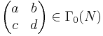
Let $N$ be a positive integer. The modular group Γ₀(N) is defined as

$\Gamma_0(N) = \left\{ \begin{pmatrix} a & b \\ c & d \end{pmatrix} \in SL_2(\mathbf{Z})�: c \equiv 0 \pmod{N} \right\}.$

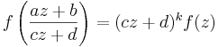
Let $k$ be a positive integer. An modular form of weight $k$ with level $N$ (or level group $\Gamma_0(N)$ ) is a holomorphic function $f$ on the upper half-plane such that for any

$\begin{pmatrix} a & b \\ c & d \end{pmatrix} \in \Gamma_0(N)$

and any $z$ in the upper half-plane, we have

$f\left(\frac{az+b}{cz+d}\right) = (cz+d)^k f(z)$

and $f$ is meromorphic at the cusp. By "meromorphic at the cusp", it is meant that the modular form is meromorphic as $z\rightarrow i\infty$ .

Note that 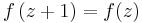$f\left(z+1\right) = f(z)$ , so modular forms are periodic, with period 1, and thus have a Fourier series.

q-expansion

The q-expansion^[1] of a modular form is the Laurent series at the cusp. Equivalently, the Fourier series, written as a Laurent series in terms of $q=\exp(2\pi iz)$ (the square of the nome).

Since $\exp$ is non-vanishing, $q \neq 0$ on the complex plane, but in the limit, $\exp(w) \to 0$ as $w \to -\infty$ (along the negative real axis), so $q \to 0$ as $2\pi iz \to -\infty$ , so as $z \to i\infty$ (along the positive imaginary axis) — thus the q-expansion is the Laurent series expansion at the cusp.

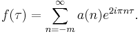
"Meromorphic at the cusp" means that only finitely many negative Fourier coefficients are non-zero, so the q-expansion is bounded below, and meromorphic at $q=0$ :

$f(z)=\sum_{n=-m}^\infty c_n \exp(2\pi inz) = \sum_{n=-m}^\infty c_n q^n.$

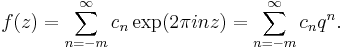
The coefficients $c_n$ are the Fourier coefficients of $f$ , and the number m is the order of the pole of f at $i\infty$ .

Entire forms, cusp forms

If $f$ is holomorphic at the cusp (has no pole at $q=0$ ), it is called an entire modular form.

If $f$ is meromorphic but not holomorphic at the cusp, it is called a non-entire modular form. For example, the j-invariant is a non-entire modular form of weight 0, and has a simple pole at $i\infty$ .

If $f$ is entire and vanishes at $q=0$ (so $c_0=0$ ), the form is called a cusp form (Spitzenform in German). The smallest n such that $c_n \ne 0$ is the order of the zero of f at $i\infty$ .

Automorphic factors and other generalizations

Other common generalizations allow the weight k to not be an integer, and allow a multiplier $\epsilon(a,b,c,d)$ with $\left|\varepsilon(a,b,c,d)\right|=1$ to appear in the transformation, so that

$f\left(\frac{az+b}{cz+d}\right) = \varepsilon(a,b,c,d) (cz+d)^k f(z).$

Functions of the form $\epsilon(a,b,c,d) (cz+d)^k$ are known as automorphic factors.

By allowing automorphic factors, functions such as the Dedekind eta function may be encompassed by the theory, being a modular form of weight 1/2. Thus, for example, let $\chi$ be a Dirichlet character mod $N$ . A modular form of weight $k$ , level $N$ (or level group $\Gamma_0(N)$ ) with nebentypus $\chi$ is a holomorphic function $f$ on the upper half-plane such that for any

$\begin{pmatrix} a & b \\ c & d \end{pmatrix} \in \Gamma_0(N)$

and any $z$ in the upper half-plane, we have

$f\left(\frac{az+b}{cz+d}\right) = \chi(d)(cz+d)^k f(z)$

and $f$ is holomorphic at the cusp. Sometimes the convention

$\chi^{-1}(d) (cz+d)^k f(z)$

is used for the right hand side of the above equation.

Examples

The simplest examples from this point of view are the Eisenstein series. For each even integer k > 2, we define E_k(Λ) to be the sum of λ^−k over all non-zero vectors λ of Λ:

$E_k(\Lambda) = \sum_{\lambda\in\Lambda-0}\lambda^{-k}.$

The condition k > 2 is needed for convergence; the condition that k is even prevents λ^−k from cancelling with (−λ)^−k.

An even unimodular lattice L in Rⁿ is a lattice generated by n vectors forming the columns of a matrix of determinant 1 and satisfying the condition that the square of the length of each vector in L is an even integer. As a consequence of the Poisson summation formula, the theta function

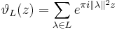
$\vartheta_L(z) = \sum_{\lambda\in L}e^{\pi i \Vert\lambda\Vert^2 z}$

is a modular form of weight n/2. It is not so easy to construct even unimodular lattices, but here is one way: Let n be an integer divisible by 8 and consider all vectors v in Rⁿ such that 2v has integer coordinates, either all even or all odd, and such that the sum of the coordinates of v is an even integer. We call this lattice L_n. When n=8, this is the lattice generated by the roots in the root system called E₈. Because there is only one modular form of weight 8 up to scalar multiplication,

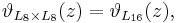
$\vartheta_{L_8\times L_8}(z) = \vartheta_{L_{16}}(z),$

even though the lattices L₈×L₈ and L₁₆ are not similar. John Milnor observed that the 16-dimensional tori obtained by dividing R¹⁶ by these two lattices are consequently examples of compact Riemannian manifolds which are isospectral but not isometric (see Hearing the shape of a drum.)

The Dedekind eta function is defined as

$\eta(z) = q^{1/24}\prod_{n=1}^\infty (1-q^n),\ q = e^{2\pi i z}.$

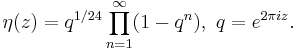
Then the modular discriminant Δ(z)=η(z)²⁴ is a modular form of weight 12. A celebrated conjecture of Ramanujan asserted that the q^p coefficient for any prime p has absolute value ≤2p^11/2. This was settled by Pierre Deligne as a result of his work on the Weil conjectures.

The second and third examples give some hint of the connection between modular forms and classical questions in number theory, such as representation of integers by quadratic forms and the partition function. The crucial conceptual link between modular forms and number theory are furnished by the theory of Hecke operators, which also gives the link between the theory of modular forms and representation theory.

Generalizations

There are various notions of modular form more general than the one discussed above. The assumption of complex analyticity can be dropped; Maass forms are real-analytic eigenfunctions of the Laplacian but need not be holomorphic. The holomorphic parts of certain weak Maass wave forms turn out to be essentially Ramanujan's mock theta functions. Groups which are not subgroups of SL₂(Z) can be considered. Hilbert modular forms are functions in n variables, each a complex number in the upper half-plane, satisfying a modular relation for 2×2 matrices with entries in a totally real number field. Siegel modular forms are associated to larger symplectic groups in the same way in which the forms we have discussed are associated to SL₂(R); in other words, they are related to abelian varieties in the same sense that our forms (which are sometimes called elliptic modular forms to emphasize the point) are related to elliptic curves. Automorphic forms extend the notion of modular forms to general Lie groups.

History

The theory of modular forms was developed in three or four periods: first in connection with the theory of elliptic functions, in the first part of the nineteenth century; then by Felix Klein and others towards the end of the nineteenth century as the automorphic form concept became understood (for one variable); then by Erich Hecke from about 1925; and then in the 1960s, as the needs of number theory and the formulation of the modularity theorem in particular made it clear that modular forms are deeply implicated.

The term modular form, as a systematic description, is usually attributed to Hecke.

Notes

↑ Elliptic and Modular Functions

References

Jean-Pierre Serre: A Course in Arithmetic. Graduate Texts in Mathematics 7, Springer-Verlag, New York, 1973. Chapter VII provides an elementary introduction to the theory of modular forms.
Tom M. Apostol, Modular functions and Dirichlet Series in Number Theory (1990), Springer-Verlag, New York. ISBN 0-387-97127-0
Goro Shimura: Introduction to the arithmetic theory of automorphic functions. Princeton University Press, Princeton, N.J., 1971. Provides a more advanced treatment.
Stephen Gelbart: Automorphic forms on adele groups. Annals of Mathematics Studies 83, Princeton University Press, Princeton, N.J., 1975. Provides an introduction to modular forms from the point of view of representation theory.
Robert A. Rankin, Modular forms and functions, (1977) Cambridge University Press, Cambridge. ISBN 0-521-21212-X
Stein's notes on Ribet's course Modular Forms and Hecke Operators